Distributed Computing Basic Note - 1

Introduction

This blog introduces basic types of parallel computing architecture, memory, and basic evaluation metrics of parallel computing.

Parallel Computing

1. Features of Parallel computing

• Features of Problem:

  • problem task can be broken into discrete pieces of work
  • Problem can be solved faster with multiple computing resource than single resource

• Features of Computing resource

  • Single computer with multiple processors
  • Multiple computers connected in network
  • Combine 1,2
  • Special computing component (GPU)

• Execution

  • Execute multiple instructions concurrently in time

2. Relationship between Parallel, Distributed, Cluster, Concurrency Computing:
   $ Cluster Computing \subset Distributed Computing \subset Parallel computing \subset Concurrencty Computing$

Evaluation of Computing performance

Amdahl’s Law

Assume:
$f_s$: fraction that the program is not parallelizable (the ratio of series part to whole program)
Or called portion of series in the program
p: Number of processor
$t_p$: runtime of parallelizable operation
$t_s$: runtime of series operation
S(p): Parallel Speedup
Then
Amdahl’s Law: $t_p = f_s S(p) + \frac{(1-p)f_s}{p} $

Parallel Speedup

Parallel Speedup: $S(p) = \frac{t_s}{t_p} = \frac{p}{(p-1)*f+1}$. Usually Parallel Speedup $S(p) \leq p$

Limiting Factors affecting Parallel Speedup:

1. Not parallelizable code (or Series operation runtime): $t_s$. Longer runtime series code takes, larger $f_s$ is and Smaller the Parallel Efficiency is

2. Communication Overhead: more time is spent on communication, then it also increases $t_s$

Parallel Efficiency

Parallel Efficiency: $E = \frac{S(p)}{p} = \frac{1}{(p-1)*f + 1}$
Parallel Efficiency measures how efficient the parallelization is. Higher Efficiency is, more busy each processor is and Faster the operations are executed.

So we want to increase parallel Efficiency and maximize the ratio between S(p) and p.

Type of Parallel Speedup

1. Linear Speedup (normal case): $S(p) < p$
2. Sublinear Speedup: $S(p) = p$
3. Superlinear Speedup: $S(p) > p$

limiting Factors lead to superlilnear Speedup:

1. Poor sequential reference implementation, leading to $t_s$ very large and series runtime very large

2. Memory caching: when memory cache is small, it will increase $t_s$ and lead to lower processing speed such that $t_s >t_p$ and S(p) >p
3. I/O blocking : block I/O leads to delay of runtime, $t_s$ will increase

Types of Computers

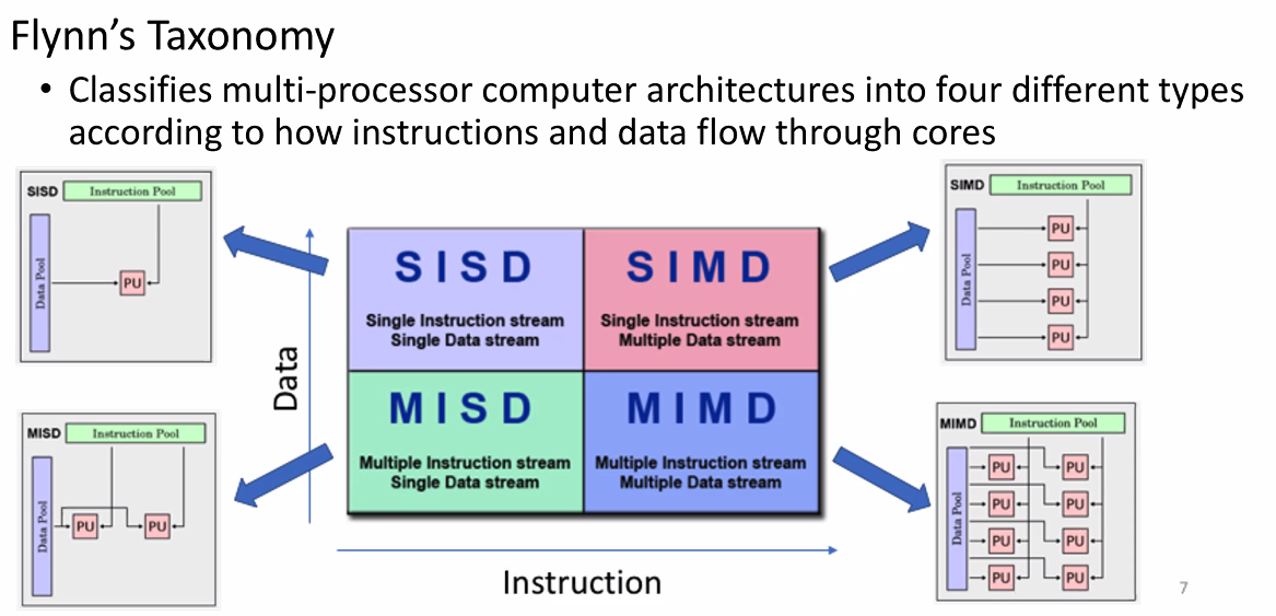
Flynne’s Taxonomy

This taxonomy classifies the computer architecture into four types:

• SISD: Single Instruction Single Datastream
• SIMD: Single Instruction Multiple Datastreams
• MISD: Multiple Instructions Single Datastream
• MIMD: Multiple Instructions Multiple Datastreams

Note:

• SIMD, MISD, MIMD architecture belongs to parallel computer since they satisfy the requirements of feature in parallel computing ( break task into piece, execute multiple(same or different )instrutions concurrently, etc)

Type of Memory

1. Shared Memory
   Multiple processors share the same memory
2. Distributed Memory and Message Passing
   Multiple processors have its own memory but use message passing method to communicate with each other distributedly across network.
3. Hyper-Model
   Combining Shared memory and distributed Memory together.

Heterogeneous computing (accelerators)

1. GPU
2. FPGA

Benchmarking and Ranking supercomputers

1. LINPACK (Linear Algebra Package): Dense Matrix Solver
2. HPCC: High-Performance Computing Challenge
3. SHOC: Scalable Heterogeneous Computing - Non-traditional systems (GPU)
4. TestDFSIO - I/O Performance of MapReduce/Hadoop Distributed File System