2020-11-22Statistic12 minutes read (About 1734 words) 0 visits

Statistic-P-value

Introduction

This article introduces how to compute the P-value using different distributions / statistic methods, including Z-distribution, t-distribution, F-test ,Chi-Square $X^2$ Distribution.
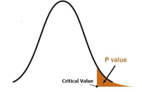
In all distributions, we first determine the random variable value in possibility density function (CDF) and then use the corresponding distribution look-up table to check the P-value (Possibility) of that distribution. Finally compare P-value with the significant level, $\alpha$ to check should we reject Null hypothesis H0 or not.

Notations

Before talking about different testing for P-value, let’s denote some notations:

x: sampled data , a small group of observations
P: population size. Population is the total set of observations that can be made
n: sample size
$\mu_0$: population mean
$\sigma_0$: population variance
$\mu’$: sample mean
$\sigma’$: sample variance

Z-test / Z-statistic (standard normal distribution)

Assumption
Z-test assumes distributions of both population and sample are Normal distribution
Null Hypothesis in z-test is that two groups have no difference
Computation of Z-Score of continuous random variable

$$
z-score = \frac{\mu’ - \mu_0 }{\sigma_0/ \sqrt{n}}
$$

if we don’t know population standard variance, but know population mean only, we can use sample variance deviation to estimate the population variance deviation. Then it becomes

$$
z-score = \frac{\mu’ - \mu_0 }{\sigma’/ \sqrt{n}}
$$

if compare two groups:

$$
z-score = \frac{\mu_1 - \mu_2 }{\sqrt{(\sigma_1^2/n_1)+(\sigma_2^2/n_2)}}
$$

Computation of Z-Score of binary random variable
Denote $p_0$ as the Population possibility of obtaining current case X, $p’$ as the Sample possibility of current case X

$$
z score = \frac{p’ - p_0 }{ (p_0(1-p_0))/ \sqrt{n}}
$$

When to use
- when we know the population is normal distribution
- when the sample size is small, usually smaller than 30.
- When we know some distribution settings, like $\mu_0$ = 0, $\sigma_0$=1 in standard normal distribution
Example
To test if two groups have no difference, we can let sample mean, variance of group A as $\mu_A$ $\sigma_A$, sample mean of group B as $\mu_B$, $\sigma_B$. Then let $\mu’ = \mu_A - \mu_B$ if we assume population mean of group difference is $\mu_0$ = 0, then we can model the group difference like this

$$
z-score = \frac{(\mu_A - \mu_B) - 0 }{\sigma_0/ \sqrt{n}}
$$

$$
z-score = \frac{(\mu_A - \mu_B) - 0 }{\sqrt{(\sigma_1^2/n_1)}}
$$

t-test / t-statistic (similar to normal distribution)

Assumption
t-test also assumes Normal distribution as the population distribution and sample distribution. Different from z-test, t-test doesn’t assume we know the parameters (mean, variance) of normal distribution..

Null Hypothesis in t-test is that two groups have no difference

Note that as degree of freedom in t-distribution increases, it is more similar to normal distribution.

Computation of t-Score for continuous random variable

$$
t-score = \frac{\mu_1 - \mu_2}{\sqrt{(\sigma_1^2/n_1)+(\sigma_2^2/n_2)}}
$$

since both t-test and z-test assume normal distribution, they have the same formula

Find P-value of t-score
After we determine the t-score in CDF, we can find the corresponding P-value in t-distribution using this table
When to use
- t-test is used when population parameters (population mean and population variance) are not known
- when sample size is very large, usually >30. (So usually in model evaluation, we use t-test with large dataset)
- when we assume data is normal distribution
- Note that since in t-test we don’t know the population distribution parameters, so the variances in t-test are sample variance. But in Z-test, we know the population distribution parameters, we usually use population variance and population mean instead
- In my word, z-test assumes we know normal distribution parameters, so we can use those parameters for testing and use less samples. But t-test doesn’t assume we know anything about distribution, so it uses samples parameters (sample mean and variance) to estimate the normal distribution for testing.

Chi-Square-test / $X^2$-statistic

Assumption
In Chi-Square test, it is to test the independence/correlation between categorical variables
Note that Chi-Square test is a one(right)-tail test and the we can not use it for two-tail test. It meausres the correlation of two categorical variable.

Null Hypothesis in Chi-Square test is that two groups are independent from each other

Computation of Pearson’s Chi-Square value
Consider we have two binary categorical variable with total sample size of n. The table is shown as follow, we want to test their correlation.

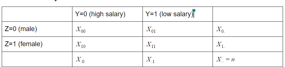
Then the Pearson’s Chi-Square Correlation is computed by

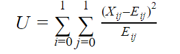
where i, j mean the $i^{th}$ row and $j^{th}$ column. n is the total sample amount
$$
E_{i,j} = \frac{X_iX_j}{n}
$$

Find P-value from Chi-Square CDF function based on the Chi Square-value we find

We can find the Chi-square distribution in this link
and the distribution table from here

When to use
- when we are testing categorical variable and we need one-tail test only
- when we are testing independence between two variables
Example:
Measuring the independence between gender and salary, independence between smoking and cancer.

F-test / F-statistic

Assumption
F-score is to measure the ratio between explained variance over the unexplained variance
Computation of F-Score for P-Value
To understand the F-score, let consider a real linear regression model:

$$
y = \beta_0 + \beta_1X_1 + \beta_2X_2 + \epsilon
$$

and an estimated linear regression
$$
y’ = \beta_0 + \beta_1X_1 + \beta_2X_2
$$
where $\epsilon$ is the unexplainable, irreducible error

Then the Residual Sum Square Error (RSS) between two linear models among n samples is

$$
RSS = \sum_i^n(y_i - y’_i)^2
$$

RSS Error is to measure the variability between two model.

In F-statistic, we want to check if there is relationship between feature $X_i$ and target. If there is no relationship, then weight $\beta_i$ = 0.(i>0).

Then Null hypothesis in F-statistic is that $\beta_1 = \beta_2=..=\beta_p=0$ consider there is no relationship between features and target
Then alternative hypothesis is that $\beta_i \neq 0$ for some i>0.

In this case, for null hypothesis, we have a Restricted Linear Model
$$
\bar{y} = \beta_0
$$

and a Full Linear model

$$
y_i’ = \beta_0 + \beta_1X_{1i}
$$

where $X_{1i}$, $\bar{y_i}$ means the the $1^{st}$ feature in the $i^{th}$ sample and the prediction of the $i^{th}$ sample.

Denote the degree of freedom of restrict model as $df_r$, and the degree of freedom of Full model as $df_F$. There are n sample data points and p+1 weight cofficients $\beta_i$ ($\beta_0$ to $\beta_p$ )to pick. Then degree of freedom = n -p.
Hence in this case, we care about choosing $\beta_1$ or not. We have $df_r$ = n-1 and $df_F$ = n-2

Total Sum Square Error (TSS) of Restrict Linear model:
$$
TSS = \sum_i^n(y_i - \bar{y})^2
$$

Residual Sum Square Error (RSS) of Full Linear model:
$$
RSS = \sum_i^n(y_i - y’_i)^2
$$

The formula to compute F-score is

$$
F-score = \frac{ (TSS-RSS)/(df_r - df_F)}{RSS/df_F} = \frac{ (TSS-RSS)/1}{RSS/(n-2)}
$$

More general, If there are p+1 weight coefficient in Full model, then we have
$$
F-score = \frac{ (TSS-RSS)/p}{RSS/(n-p-1)}
$$

where $TSS- RSS$ is the variability explained by model and $RSS$ measure the variability left unexplained after the regression (which is also the irreducible error mentioned before)

If F-value > 0 and <= 1, we don’t reject H0. If F-value >1, then we reject H0 and choose H1.
If F-value <0, then F-test fails, it doesn’t mean anything.
Note that F-test is also a One-tail hypothesis test.

When to use
- when we are measuring if some features matters in prediction / there is correlation between features and target
- F-test can be adjusted by the number of predictors, but individual t-test doesn’t
- Note that when the number of predictors p > the number of samples n, F-test will fail since value $RSS/(n-p-1)$ becomes negative and this F-value is out of the range of random variable value in F-distribution
Example
There are some examples from this link: https://online.stat.psu.edu/stat501/lesson/6/6.2

$R^2$ test

Assumption
$R^2$ measures the proportion of variability of prediction y that can be explained by feature X
Computation of $R^2$-Score for P-Value
$$
R^2 - value = \frac{TSS- RSS}{RSS}
$$

where RSS and TSS are computed as same as those in F-test

$$
TSS = \sum_i^n(y_i - \bar{y})^2
$$

where $\bar{y} =\beta_0$ = mean of $y_i$
since when we estimate $\bar{y} =\beta_0$ using samples to minimize the sum square loss, let gradient of $\sum_i^n(y_i-\bar{y})^2$ = 0, we have $-2\sum_i^n(y_i-\bar{y}) =0$ and $\bar{y} = (\sum_i^ny_i)/n$

Residual Sum Square Error (RSS) of Full Linear model:
$$
RSS = \sum_i^n(y_i - y’_i)^2
$$

Random Variable $R^2$ has range [0,1]. If $R^2$ fall outside this range, then the test fails. If $R^2$ value is close to 1, then reject H0 and consider H1 and there is relationship between features and y. if $R^2$ value is close to 0, then model is wrong and don’t fit well, then can not reject H0.