1
2
from google.colab import drivedrive.mount('/content/drive' )
Drive already mounted at /content/drive; to attempt to forcibly remount, call drive.mount("/content/drive", force_remount=True).
Requirement already satisfied: kaggle in /usr/local/lib/python3.6/dist-packages (1.5.9)
Requirement already satisfied: python-slugify in /usr/local/lib/python3.6/dist-packages (from kaggle) (4.0.1)
Requirement already satisfied: python-dateutil in /usr/local/lib/python3.6/dist-packages (from kaggle) (2.8.1)
Requirement already satisfied: six>=1.10 in /usr/local/lib/python3.6/dist-packages (from kaggle) (1.15.0)
Requirement already satisfied: certifi in /usr/local/lib/python3.6/dist-packages (from kaggle) (2020.11.8)
Requirement already satisfied: urllib3 in /usr/local/lib/python3.6/dist-packages (from kaggle) (1.24.3)
Requirement already satisfied: slugify in /usr/local/lib/python3.6/dist-packages (from kaggle) (0.0.1)
Requirement already satisfied: tqdm in /usr/local/lib/python3.6/dist-packages (from kaggle) (4.41.1)
Requirement already satisfied: requests in /usr/local/lib/python3.6/dist-packages (from kaggle) (2.23.0)
Requirement already satisfied: text-unidecode>=1.3 in /usr/local/lib/python3.6/dist-packages (from python-slugify->kaggle) (1.3)
Requirement already satisfied: idna<3,>=2.5 in /usr/local/lib/python3.6/dist-packages (from requests->kaggle) (2.10)
Requirement already satisfied: chardet<4,>=3.0.2 in /usr/local/lib/python3.6/dist-packages (from requests->kaggle) (3.0.4)
1 !cp /content/drive/My\ Drive/Colab\ Notebooks/KKBox-MusicRecommendationSystem/kaggle.json .
1 2 3 4 5 6 7 !mkdir -p ~/.kaggle !cp kaggle.json ~/.kaggle/ !ls ~/.kaggle !mkdir -p ./kaggle/ !chmod 600 /root/.kaggle/kaggle.json !kaggle competitions download kkbox-music-recommendation-challenge
kaggle.json
Warning: Looks like you're using an outdated API Version, please consider updating (server 1.5.9 / client 1.5.4)
song_extra_info.csv.7z: Skipping, found more recently modified local copy (use --force to force download)
train.csv.7z: Skipping, found more recently modified local copy (use --force to force download)
test.csv.7z: Skipping, found more recently modified local copy (use --force to force download)
songs.csv.7z: Skipping, found more recently modified local copy (use --force to force download)
members.csv.7z: Skipping, found more recently modified local copy (use --force to force download)
sample_submission.csv.7z: Skipping, found more recently modified local copy (use --force to force download)
1
2
3
4
5
6
7
8
9
10
11
12
!mkdir kaggle/working !mkdir kaggle/working/train !mkdir kaggle/working/train/data !apt-get install p7zip !apt-get install p7zip-full !7 za e members.csv.7 z !7 za e songs.csv.7 z !7 za e song_extra_info.csv.7 z !7 za e train.csv.7 z !7 za e sample_submission.csv.7 z !7 za e test.csv.7 z !mv *.csv kaggle/working/train/data
mkdir: cannot create directory ‘kaggle/working’: File exists
mkdir: cannot create directory ‘kaggle/working/train’: File exists
mkdir: cannot create directory ‘kaggle/working/train/data’: File exists
Reading package lists... Done
Building dependency tree
Reading state information... Done
p7zip is already the newest version (16.02+dfsg-6).
0 upgraded, 0 newly installed, 0 to remove and 14 not upgraded.
Reading package lists... Done
Building dependency tree
Reading state information... Done
p7zip-full is already the newest version (16.02+dfsg-6).
0 upgraded, 0 newly installed, 0 to remove and 14 not upgraded.
7-Zip (a) [64] 16.02 : Copyright (c) 1999-2016 Igor Pavlov : 2016-05-21
p7zip Version 16.02 (locale=en_US.UTF-8,Utf16=on,HugeFiles=on,64 bits,2 CPUs AMD EPYC 7B12 (830F10),ASM,AES-NI)
Scanning the drive for archives:
0M Scan��������� ���������1 file, 1349856 bytes (1319 KiB)
Extracting archive: members.csv.7z
--
Path = members.csv.7z
Type = 7z
Physical Size = 1349856
Headers Size = 130
Method = LZMA2:3m
Solid = -
Blocks = 1
0%���� ����Everything is Ok
Size: 2503827
Compressed: 1349856
7-Zip (a) [64] 16.02 : Copyright (c) 1999-2016 Igor Pavlov : 2016-05-21
p7zip Version 16.02 (locale=en_US.UTF-8,Utf16=on,HugeFiles=on,64 bits,2 CPUs AMD EPYC 7B12 (830F10),ASM,AES-NI)
Scanning the drive for archives:
0M Scan��������� ���������1 file, 105809525 bytes (101 MiB)
Extracting archive: songs.csv.7z
--
Path = songs.csv.7z
Type = 7z
Physical Size = 105809525
Headers Size = 122
Method = LZMA2:24
Solid = -
Blocks = 1
0%���� ���� 2% - songs.csv���������������� ���������������� 5% - songs.csv���������������� ���������������� 8% - songs.csv���������������� ���������������� 11% - songs.csv���������������� ���������������� 14% - songs.csv���������������� ���������������� 17% - songs.csv���������������� ���������������� 20% - songs.csv���������������� ���������������� 24% - songs.csv���������������� ���������������� 27% - songs.csv���������������� ���������������� 30% - songs.csv���������������� ���������������� 33% - songs.csv���������������� ���������������� 35% - songs.csv���������������� ���������������� 39% - songs.csv���������������� ���������������� 41% - songs.csv���������������� ���������������� 45% - songs.csv���������������� ���������������� 49% - songs.csv���������������� ���������������� 51% - songs.csv���������������� ���������������� 54% - songs.csv���������������� ���������������� 57% - songs.csv���������������� ���������������� 60% - songs.csv���������������� ���������������� 62% - songs.csv���������������� ���������������� 65% - songs.csv���������������� ���������������� 68% - songs.csv���������������� ���������������� 70% - songs.csv���������������� ���������������� 73% - songs.csv���������������� ���������������� 76% - songs.csv���������������� ���������������� 79% - songs.csv���������������� ���������������� 82% - songs.csv���������������� ���������������� 85% - songs.csv���������������� ���������������� 87% - songs.csv���������������� ���������������� 90% - songs.csv���������������� ���������������� 92% - songs.csv���������������� ���������������� 95% - songs.csv���������������� ���������������� 98% - songs.csv���������������� ����������������Everything is Ok
Size: 221828666
Compressed: 105809525
7-Zip (a) [64] 16.02 : Copyright (c) 1999-2016 Igor Pavlov : 2016-05-21
p7zip Version 16.02 (locale=en_US.UTF-8,Utf16=on,HugeFiles=on,64 bits,2 CPUs AMD EPYC 7B12 (830F10),ASM,AES-NI)
Scanning the drive for archives:
0M Scan��������� ���������1 file, 103608205 bytes (99 MiB)
Extracting archive: song_extra_info.csv.7z
--
Path = song_extra_info.csv.7z
Type = 7z
Physical Size = 103608205
Headers Size = 140
Method = LZMA:25
Solid = -
Blocks = 1
0%���� ���� 1% - song_extra_info.csv�������������������������� �������������������������� 4% - song_extra_info.csv�������������������������� �������������������������� 6% - song_extra_info.csv�������������������������� �������������������������� 9% - song_extra_info.csv�������������������������� �������������������������� 11% - song_extra_info.csv�������������������������� �������������������������� 13% - song_extra_info.csv�������������������������� �������������������������� 16% - song_extra_info.csv�������������������������� �������������������������� 18% - song_extra_info.csv�������������������������� �������������������������� 20% - song_extra_info.csv�������������������������� �������������������������� 23% - song_extra_info.csv�������������������������� �������������������������� 25% - song_extra_info.csv�������������������������� �������������������������� 27% - song_extra_info.csv�������������������������� �������������������������� 30% - song_extra_info.csv�������������������������� �������������������������� 32% - song_extra_info.csv�������������������������� �������������������������� 34% - song_extra_info.csv�������������������������� �������������������������� 37% - song_extra_info.csv�������������������������� �������������������������� 39% - song_extra_info.csv�������������������������� �������������������������� 41% - song_extra_info.csv�������������������������� �������������������������� 44% - song_extra_info.csv�������������������������� �������������������������� 46% - song_extra_info.csv�������������������������� �������������������������� 48% - song_extra_info.csv�������������������������� �������������������������� 50% - song_extra_info.csv�������������������������� �������������������������� 53% - song_extra_info.csv�������������������������� �������������������������� 55% - song_extra_info.csv�������������������������� �������������������������� 57% - song_extra_info.csv�������������������������� �������������������������� 60% - song_extra_info.csv�������������������������� �������������������������� 62% - song_extra_info.csv�������������������������� �������������������������� 65% - song_extra_info.csv�������������������������� �������������������������� 68% - song_extra_info.csv�������������������������� �������������������������� 71% - song_extra_info.csv�������������������������� �������������������������� 74% - song_extra_info.csv�������������������������� �������������������������� 76% - song_extra_info.csv�������������������������� �������������������������� 78% - song_extra_info.csv�������������������������� �������������������������� 81% - song_extra_info.csv�������������������������� �������������������������� 83% - song_extra_info.csv�������������������������� �������������������������� 85% - song_extra_info.csv�������������������������� �������������������������� 88% - song_extra_info.csv�������������������������� �������������������������� 92% - song_extra_info.csv�������������������������� �������������������������� 95% - song_extra_info.csv�������������������������� �������������������������� 99% - song_extra_info.csv�������������������������� ��������������������������Everything is Ok
Size: 181010294
Compressed: 103608205
7-Zip (a) [64] 16.02 : Copyright (c) 1999-2016 Igor Pavlov : 2016-05-21
p7zip Version 16.02 (locale=en_US.UTF-8,Utf16=on,HugeFiles=on,64 bits,2 CPUs AMD EPYC 7B12 (830F10),ASM,AES-NI)
Scanning the drive for archives:
0M Scan��������� ���������1 file, 106420688 bytes (102 MiB)
Extracting archive: train.csv.7z
--
Path = train.csv.7z
Type = 7z
Physical Size = 106420688
Headers Size = 122
Method = LZMA2:24
Solid = -
Blocks = 1
0%���� ���� 2% - train.csv���������������� ���������������� 4% - train.csv���������������� ���������������� 6% - train.csv���������������� ���������������� 9% - train.csv���������������� ���������������� 10% - train.csv���������������� ���������������� 13% - train.csv���������������� ���������������� 14% - train.csv���������������� ���������������� 17% - train.csv���������������� ���������������� 19% - train.csv���������������� ���������������� 21% - train.csv���������������� ���������������� 23% - train.csv���������������� ���������������� 25% - train.csv���������������� ���������������� 27% - train.csv���������������� ���������������� 29% - train.csv���������������� ���������������� 31% - train.csv���������������� ���������������� 33% - train.csv���������������� ���������������� 34% - train.csv���������������� ���������������� 36% - train.csv���������������� ���������������� 38% - train.csv���������������� ���������������� 41% - train.csv���������������� ���������������� 43% - train.csv���������������� ���������������� 46% - train.csv���������������� ���������������� 48% - train.csv���������������� ���������������� 50% - train.csv���������������� ���������������� 52% - train.csv���������������� ���������������� 54% - train.csv���������������� ���������������� 56% - train.csv���������������� ���������������� 58% - train.csv���������������� ���������������� 59% - train.csv���������������� ���������������� 62% - train.csv���������������� ���������������� 65% - train.csv���������������� ���������������� 68% - train.csv���������������� ���������������� 70% - train.csv���������������� ���������������� 73% - train.csv���������������� ���������������� 75% - train.csv���������������� ���������������� 76% - train.csv���������������� ���������������� 78% - train.csv���������������� ���������������� 80% - train.csv���������������� ���������������� 82% - train.csv���������������� ���������������� 84% - train.csv���������������� ���������������� 86% - train.csv���������������� ���������������� 88% - train.csv���������������� ���������������� 90% - train.csv���������������� ���������������� 91% - train.csv���������������� ���������������� 93% - train.csv���������������� ���������������� 95% - train.csv���������������� ���������������� 97% - train.csv���������������� ���������������� 99% - train.csv���������������� ����������������Everything is Ok
Size: 971675848
Compressed: 106420688
7-Zip (a) [64] 16.02 : Copyright (c) 1999-2016 Igor Pavlov : 2016-05-21
p7zip Version 16.02 (locale=en_US.UTF-8,Utf16=on,HugeFiles=on,64 bits,2 CPUs AMD EPYC 7B12 (830F10),ASM,AES-NI)
Scanning the drive for archives:
0M Scan��������� ���������1 file, 463688 bytes (453 KiB)
Extracting archive: sample_submission.csv.7z
--
Path = sample_submission.csv.7z
Type = 7z
Physical Size = 463688
Headers Size = 146
Method = LZMA2:24
Solid = -
Blocks = 1
0%���� ����Everything is Ok
Size: 29570380
Compressed: 463688
7-Zip (a) [64] 16.02 : Copyright (c) 1999-2016 Igor Pavlov : 2016-05-21
p7zip Version 16.02 (locale=en_US.UTF-8,Utf16=on,HugeFiles=on,64 bits,2 CPUs AMD EPYC 7B12 (830F10),ASM,AES-NI)
Scanning the drive for archives:
0M Scan��������� ���������1 file, 43925208 bytes (42 MiB)
Extracting archive: test.csv.7z
--
Path = test.csv.7z
Type = 7z
Physical Size = 43925208
Headers Size = 122
Method = LZMA2:24
Solid = -
Blocks = 1
0%���� ���� 4% - test.csv��������������� ��������������� 8% - test.csv��������������� ��������������� 13% - test.csv��������������� ��������������� 18% - test.csv��������������� ��������������� 22% - test.csv��������������� ��������������� 28% - test.csv��������������� ��������������� 34% - test.csv��������������� ��������������� 42% - test.csv��������������� ��������������� 49% - test.csv��������������� ��������������� 55% - test.csv��������������� ��������������� 61% - test.csv��������������� ��������������� 67% - test.csv��������������� ��������������� 74% - test.csv��������������� ��������������� 80% - test.csv��������������� ��������������� 86% - test.csv��������������� ��������������� 90% - test.csv��������������� ��������������� 96% - test.csv��������������� ���������������Everything is Ok
Size: 347789925
Compressed: 43925208
1 2 3 4 5 6 7 8 9 10 11 12 13 14 15 16 17 import numpy as np import pandas as pd import osfor dirname, _, filenames in os.walk('./kaggle/input' ): for filename in filenames: print(os.path.join(dirname, filename))
Use 7z to uncompress the csv files 1 !ls ./kaggle/working/train/data/
members.csv           song_extra_info.csv  test.csv
sample_submission.csv  songs.csv        train.csv
1 !du -h ./kaggle/working/train/data/
1.7G ./kaggle/working/train/data/
processor    : 0
vendor_id    : AuthenticAMD
cpu family    : 23
model        : 49
model name    : AMD EPYC 7B12
stepping    : 0
microcode    : 0x1000065
cpu MHz        : 2250.000
cache size    : 512 KB
physical id    : 0
siblings    : 2
core id        : 0
cpu cores    : 1
apicid        : 0
initial apicid    : 0
fpu        : yes
fpu_exception    : yes
cpuid level    : 13
wp        : yes
flags        : fpu vme de pse tsc msr pae mce cx8 apic sep mtrr pge mca cmov pat pse36 clflush mmx fxsr sse sse2 ht syscall nx mmxext fxsr_opt pdpe1gb rdtscp lm constant_tsc rep_good nopl xtopology nonstop_tsc cpuid extd_apicid tsc_known_freq pni pclmulqdq ssse3 fma cx16 sse4_1 sse4_2 movbe popcnt aes xsave avx f16c rdrand hypervisor lahf_lm cmp_legacy cr8_legacy abm sse4a misalignsse 3dnowprefetch osvw topoext ssbd ibrs ibpb stibp vmmcall fsgsbase tsc_adjust bmi1 avx2 smep bmi2 rdseed adx smap clflushopt clwb sha_ni xsaveopt xsavec xgetbv1 clzero xsaveerptr arat npt nrip_save umip rdpid
bugs        : sysret_ss_attrs spectre_v1 spectre_v2 spec_store_bypass
bogomips    : 4500.00
TLB size    : 3072 4K pages
clflush size    : 64
cache_alignment    : 64
address sizes    : 48 bits physical, 48 bits virtual
power management:

processor    : 1
vendor_id    : AuthenticAMD
cpu family    : 23
model        : 49
model name    : AMD EPYC 7B12
stepping    : 0
microcode    : 0x1000065
cpu MHz        : 2250.000
cache size    : 512 KB
physical id    : 0
siblings    : 2
core id        : 0
cpu cores    : 1
apicid        : 1
initial apicid    : 1
fpu        : yes
fpu_exception    : yes
cpuid level    : 13
wp        : yes
flags        : fpu vme de pse tsc msr pae mce cx8 apic sep mtrr pge mca cmov pat pse36 clflush mmx fxsr sse sse2 ht syscall nx mmxext fxsr_opt pdpe1gb rdtscp lm constant_tsc rep_good nopl xtopology nonstop_tsc cpuid extd_apicid tsc_known_freq pni pclmulqdq ssse3 fma cx16 sse4_1 sse4_2 movbe popcnt aes xsave avx f16c rdrand hypervisor lahf_lm cmp_legacy cr8_legacy abm sse4a misalignsse 3dnowprefetch osvw topoext ssbd ibrs ibpb stibp vmmcall fsgsbase tsc_adjust bmi1 avx2 smep bmi2 rdseed adx smap clflushopt clwb sha_ni xsaveopt xsavec xgetbv1 clzero xsaveerptr arat npt nrip_save umip rdpid
bugs        : sysret_ss_attrs spectre_v1 spectre_v2 spec_store_bypass
bogomips    : 4500.00
TLB size    : 3072 4K pages
clflush size    : 64
cache_alignment    : 64
address sizes    : 48 bits physical, 48 bits virtual
power management:
KKBox-Music Recommendation System Goal of this project In this project, we are going to build a recommendation system to predict the chances of a user listening to a song repetitively after the first observable listening event within a time window was triggered. If there are recurring listening event(s) triggered within a month after the user’s very first observable listening event, its target is marked 1, and 0 otherwise in the training set. The same rule applies to the testing set.
0. Data Collection and Description The KKBox dataset is composed of following files:
train.csv
msno: user id
song_id: song id
source_system_tab: the name of the tab where the event was triggered. System tabs are used to categorize KKBOX mobile apps functions. For example, tab my library contains functions to manipulate the local storage, and tab search contains functions relating to search.
source_screen_name: name of the layout a user sees.
source_type: an entry point a user first plays music on mobile apps. An entry point could be album, online-playlist, song .. etc.
target: this is the target variable. target=1 means there are recurring listening event(s) triggered within a month after the user’s very first observable listening event, target=0 otherwise .
test.csv
id: row id (will be used for submission)
msno: user id
song_id: song id
source_system_tab: the name of the tab where the event was triggered. System tabs are used to categorize KKBOX mobile apps functions. For example, tab my library contains functions to manipulate the local storage, and tab search contains functions relating to search.
source_screen_name: name of the layout a user sees.
source_type: an entry point a user first plays music on mobile apps. An entry point could be album, online-playlist, song .. etc.
sample_submission.csv
sample submission file in the format that we expect you to submit
id: same as id in test.csv
target: this is the target variable. target=1 means there are recurring listening event(s) triggered within a month after the user’s very first observable listening event, target=0 otherwise .
songs.csv
song_id
song_length: in ms
genre_ids: genre category. Some songs have multiple genres and they are separated by |
artist_name
composer
lyricist
language
members.csv
msno
city
bd: age. Note: this column has outlier values, please use your judgement.
gender
registered_via: registration method
registration_init_time: format %Y%m%d
expiration_date: format %Y%m%d
song_extra_info.csv
song_id
song name - the name of the song.
isrc - International Standard Recording Code, theoretically can be used as an identity of a song. However, what worth to note is, ISRCs generated from providers have not been officially verified; therefore the information in ISRC, such as country code and reference year, can be misleading/incorrect. Multiple songs could share one ISRC since a single recording could be re-published several times.
1. Data Cleaning and Exploratory Data Analysis (EDA)
Find the Description and summary of each CSV file and Determine Null object, categorical attributes, numerical attributes
Convert some attribute types to correct data type, like convert string to float, if necessary
Handle Missing values
Plot univariate, bivariate plots to visualize and analyze relationship between attributes and target
Analysis Summary in this section
2. Data Preprocessing Note that This section is to give some examples to preprocess data like filling missing values and removing outliers.
In order to train models, you should start from step 3 ETL to extract and transform data directly using integrated functions
4. Machine Learning Modeling
LGBM Boosting machine
In this part, we try LGBM model with different max_depth of tree: [10, 15,20, 25, 30] and see how max_depth affects the accuracy on prediction
Wide and Deep Neural network model
5. Model Training and validation
In model training and validation step, we split the data set into training set(80% of dataset) and validation set (20% of dataset) and then use them to train and keep track of the performance of models.
6. Model Evaluation In Model evaluation step, we simply use the validation set to validate the final trained models and then let models make predictions on testset from kaggle and submit predictions to kaggle to see the final evaluation scores.
7. Summary 1 2 3 4 5 6 7 8 9 10 11 12 import warningswarnings.filterwarnings('ignore' ) import numpy as np import pandas as pdimport matplotlib.pyplot as pltimport seaborn as snsimport lightgbm as lgbfrom subprocess import check_outputnp.random.seed(2020 )
1. Exploratory Data Analysis 1 2 3 4 5 6 7 8 root = './kaggle/working/train/data/' train_df = pd.read_csv(root+ "train.csv" ) test_df = pd.read_csv(root+ "test.csv" ) song_df = pd.read_csv(root+ "songs.csv" ) song_extra_df = pd.read_csv(root+ "song_extra_info.csv" ) members_df = pd.read_csv(root+ "members.csv" )
<class 'pandas.core.frame.DataFrame'>
RangeIndex: 7377418 entries, 0 to 7377417
Data columns (total 6 columns):
# Column Dtype
--- ------ -----
0 msno object
1 song_id object
2 source_system_tab object
3 source_screen_name object
4 source_type object
5 target int64
dtypes: int64(1), object(5)
memory usage: 337.7+ MB
msno 7377418
song_id 7377418
source_system_tab 7352569
source_screen_name 6962614
source_type 7355879
target 7377418
dtype: int64
We can see that attributes: source_system_tab, source_screen_name, source_type contain missing values
msno
song_id
source_system_tab
source_screen_name
source_type
target
0
FGtllVqz18RPiwJj/edr2gV78zirAiY/9SmYvia+kCg=
BBzumQNXUHKdEBOB7mAJuzok+IJA1c2Ryg/yzTF6tik=
explore
Explore
online-playlist
1
1
Xumu+NIjS6QYVxDS4/t3SawvJ7viT9hPKXmf0RtLNx8=
bhp/MpSNoqoxOIB+/l8WPqu6jldth4DIpCm3ayXnJqM=
my library
Local playlist more
local-playlist
1
2
Xumu+NIjS6QYVxDS4/t3SawvJ7viT9hPKXmf0RtLNx8=
JNWfrrC7zNN7BdMpsISKa4Mw+xVJYNnxXh3/Epw7QgY=
my library
Local playlist more
local-playlist
1
3
Xumu+NIjS6QYVxDS4/t3SawvJ7viT9hPKXmf0RtLNx8=
2A87tzfnJTSWqD7gIZHisolhe4DMdzkbd6LzO1KHjNs=
my library
Local playlist more
local-playlist
1
4
FGtllVqz18RPiwJj/edr2gV78zirAiY/9SmYvia+kCg=
3qm6XTZ6MOCU11x8FIVbAGH5l5uMkT3/ZalWG1oo2Gc=
explore
Explore
online-playlist
1
<class 'pandas.core.frame.DataFrame'>
RangeIndex: 2556790 entries, 0 to 2556789
Data columns (total 6 columns):
# Column Dtype
--- ------ -----
0 id int64
1 msno object
2 song_id object
3 source_system_tab object
4 source_screen_name object
5 source_type object
dtypes: int64(1), object(5)
memory usage: 117.0+ MB
id 2556790
msno 2556790
song_id 2556790
source_system_tab 2548348
source_screen_name 2393907
source_type 2549493
dtype: int64
In test dataset, We can see that attributes that contain missing values:
source_system_tab
source_screen_name
source_type
id
msno
song_id
source_system_tab
source_screen_name
source_type
0
0
V8ruy7SGk7tDm3zA51DPpn6qutt+vmKMBKa21dp54uM=
WmHKgKMlp1lQMecNdNvDMkvIycZYHnFwDT72I5sIssc=
my library
Local playlist more
local-library
1
1
V8ruy7SGk7tDm3zA51DPpn6qutt+vmKMBKa21dp54uM=
y/rsZ9DC7FwK5F2PK2D5mj+aOBUJAjuu3dZ14NgE0vM=
my library
Local playlist more
local-library
2
2
/uQAlrAkaczV+nWCd2sPF2ekvXPRipV7q0l+gbLuxjw=
8eZLFOdGVdXBSqoAv5nsLigeH2BvKXzTQYtUM53I0k4=
discover
NaN
song-based-playlist
3
3
1a6oo/iXKatxQx4eS9zTVD+KlSVaAFbTIqVvwLC1Y0k=
ztCf8thYsS4YN3GcIL/bvoxLm/T5mYBVKOO4C9NiVfQ=
radio
Radio
radio
4
4
1a6oo/iXKatxQx4eS9zTVD+KlSVaAFbTIqVvwLC1Y0k=
MKVMpslKcQhMaFEgcEQhEfi5+RZhMYlU3eRDpySrH8Y=
radio
Radio
radio
<class 'pandas.core.frame.DataFrame'>
RangeIndex: 2296320 entries, 0 to 2296319
Data columns (total 7 columns):
# Column Dtype
--- ------ -----
0 song_id object
1 song_length int64
2 genre_ids object
3 artist_name object
4 composer object
5 lyricist object
6 language float64
dtypes: float64(1), int64(1), object(5)
memory usage: 122.6+ MB
song_id 2296320
song_length 2296320
genre_ids 2202204
artist_name 2296320
composer 1224966
lyricist 351052
language 2296319
dtype: int64
Attributes that contain missing values are
composer
lyricist
genre_ids
language
song_id
song_length
genre_ids
artist_name
composer
lyricist
language
0
CXoTN1eb7AI+DntdU1vbcwGRV4SCIDxZu+YD8JP8r4E=
247640
465
張信哲 (Jeff Chang)
董貞
何啟弘
3.0
1
o0kFgae9QtnYgRkVPqLJwa05zIhRlUjfF7O1tDw0ZDU=
197328
444
BLACKPINK
TEDDY| FUTURE BOUNCE| Bekuh BOOM
TEDDY
31.0
2
DwVvVurfpuz+XPuFvucclVQEyPqcpUkHR0ne1RQzPs0=
231781
465
SUPER JUNIOR
NaN
NaN
31.0
3
dKMBWoZyScdxSkihKG+Vf47nc18N9q4m58+b4e7dSSE=
273554
465
S.H.E
湯小康
徐世珍
3.0
4
W3bqWd3T+VeHFzHAUfARgW9AvVRaF4N5Yzm4Mr6Eo/o=
140329
726
貴族精選
Traditional
Traditional
52.0
<class 'pandas.core.frame.DataFrame'>
RangeIndex: 2295971 entries, 0 to 2295970
Data columns (total 3 columns):
# Column Dtype
--- ------ -----
0 song_id object
1 name object
2 isrc object
dtypes: object(3)
memory usage: 52.6+ MB
song_id 2295971
name 2295969
isrc 2159423
dtype: int64
song_id
name
isrc
0
LP7pLJoJFBvyuUwvu+oLzjT+bI+UeBPURCecJsX1jjs=
我們
TWUM71200043
1
ClazTFnk6r0Bnuie44bocdNMM3rdlrq0bCGAsGUWcHE=
Let Me Love You
QMZSY1600015
2
u2ja/bZE3zhCGxvbbOB3zOoUjx27u40cf5g09UXMoKQ=
原諒我
TWA530887303
3
92Fqsy0+p6+RHe2EoLKjHahORHR1Kq1TBJoClW9v+Ts=
Classic
USSM11301446
4
0QFmz/+rJy1Q56C1DuYqT9hKKqi5TUqx0sN0IwvoHrw=
愛投羅網
TWA471306001
<class 'pandas.core.frame.DataFrame'>
RangeIndex: 34403 entries, 0 to 34402
Data columns (total 7 columns):
# Column Non-Null Count Dtype
--- ------ -------------- -----
0 msno 34403 non-null object
1 city 34403 non-null int64
2 bd 34403 non-null int64
3 gender 14501 non-null object
4 registered_via 34403 non-null int64
5 registration_init_time 34403 non-null int64
6 expiration_date 34403 non-null int64
dtypes: int64(5), object(2)
memory usage: 1.8+ MB
1 train_df['song_id' ].head()
0 BBzumQNXUHKdEBOB7mAJuzok+IJA1c2Ryg/yzTF6tik=
1 bhp/MpSNoqoxOIB+/l8WPqu6jldth4DIpCm3ayXnJqM=
2 JNWfrrC7zNN7BdMpsISKa4Mw+xVJYNnxXh3/Epw7QgY=
3 2A87tzfnJTSWqD7gIZHisolhe4DMdzkbd6LzO1KHjNs=
4 3qm6XTZ6MOCU11x8FIVbAGH5l5uMkT3/ZalWG1oo2Gc=
Name: song_id, dtype: object
1 song_df['song_id' ].head()
0 CXoTN1eb7AI+DntdU1vbcwGRV4SCIDxZu+YD8JP8r4E=
1 o0kFgae9QtnYgRkVPqLJwa05zIhRlUjfF7O1tDw0ZDU=
2 DwVvVurfpuz+XPuFvucclVQEyPqcpUkHR0ne1RQzPs0=
3 dKMBWoZyScdxSkihKG+Vf47nc18N9q4m58+b4e7dSSE=
4 W3bqWd3T+VeHFzHAUfARgW9AvVRaF4N5Yzm4Mr6Eo/o=
Name: song_id, dtype: object
1 2 3 print("Unique Song amount in trainset:" ,train_df['song_id' ].nunique()) print("Unique Song amount in testset:" , test_df['song_id' ].nunique()) print("Unique Song amount in song list:" ,song_df['song_id' ].nunique())
Unique Song amount in trainset: 359966
Unique Song amount in testset: 224753
Unique Song amount in song list: 2296320
1 2 3 4 5 user_music_df = train_df.merge(song_df,on='song_id' ,how="left" , copy =False ) user_music_df["song_id" ] = user_music_df["song_id" ].astype("category" ) user_music_df.head()
msno
song_id
source_system_tab
source_screen_name
source_type
target
song_length
genre_ids
artist_name
composer
lyricist
language
0
FGtllVqz18RPiwJj/edr2gV78zirAiY/9SmYvia+kCg=
BBzumQNXUHKdEBOB7mAJuzok+IJA1c2Ryg/yzTF6tik=
explore
Explore
online-playlist
1
206471.0
359
Bastille
Dan Smith| Mark Crew
NaN
52.0
1
Xumu+NIjS6QYVxDS4/t3SawvJ7viT9hPKXmf0RtLNx8=
bhp/MpSNoqoxOIB+/l8WPqu6jldth4DIpCm3ayXnJqM=
my library
Local playlist more
local-playlist
1
284584.0
1259
Various Artists
NaN
NaN
52.0
2
Xumu+NIjS6QYVxDS4/t3SawvJ7viT9hPKXmf0RtLNx8=
JNWfrrC7zNN7BdMpsISKa4Mw+xVJYNnxXh3/Epw7QgY=
my library
Local playlist more
local-playlist
1
225396.0
1259
Nas
N. Jones、W. Adams、J. Lordan、D. Ingle
NaN
52.0
3
Xumu+NIjS6QYVxDS4/t3SawvJ7viT9hPKXmf0RtLNx8=
2A87tzfnJTSWqD7gIZHisolhe4DMdzkbd6LzO1KHjNs=
my library
Local playlist more
local-playlist
1
255512.0
1019
Soundway
Kwadwo Donkoh
NaN
-1.0
4
FGtllVqz18RPiwJj/edr2gV78zirAiY/9SmYvia+kCg=
3qm6XTZ6MOCU11x8FIVbAGH5l5uMkT3/ZalWG1oo2Gc=
explore
Explore
online-playlist
1
187802.0
1011
Brett Young
Brett Young| Kelly Archer| Justin Ebach
NaN
52.0
1 user_music_df['song_id' ].nunique(), user_music_df['genre_ids' ].nunique()
(359966, 572)
msno 7377418
song_id 7377418
source_system_tab 7352569
source_screen_name 6962614
source_type 7355879
target 7377418
song_length 7377304
genre_ids 7258963
artist_name 7377304
composer 5701712
lyricist 4198620
language 7377268
dtype: int64
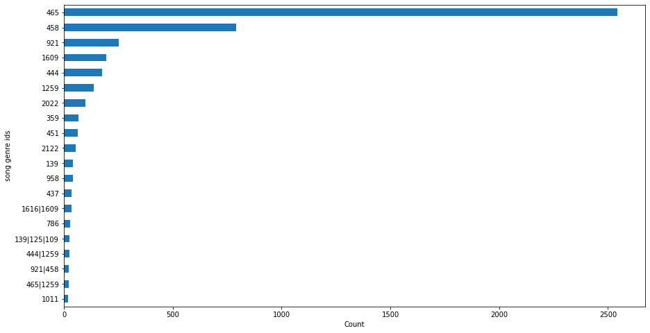
1 2 3 4 5 6 7 df_genre = user_music_df.sample(n=5000 ) df_genre = df_genre["genre_ids" ].value_counts().sort_values(ascending=False )[:20 ] df_genre = df_genre.sort_values(ascending=True ) ax = df_genre.plot.barh(figsize=(15 ,8 )) ax.set_ylabel("song genre ids" ) ax.set_xlabel("Count" )
Text(0.5, 0, 'Count')
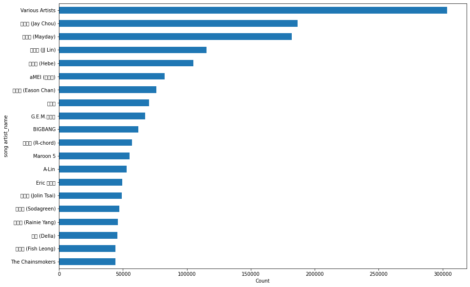
1 2 3 4 5 6 7 8 9 10 11 12 13 df_artist = user_music_df["artist_name" ].value_counts().sort_values(ascending=False )[:20 ] df_artist = df_artist.sort_values(ascending=True ) ax = df_artist.plot.barh(figsize=(15 ,10 )) ax.set_ylabel("song artist_name" ) ax.set_xlabel("Count" )
Text(0.5, 0, 'Count')
The Chainsmokers 44215
梁靜茹 (Fish Leong) 44290
丁噹 (Della) 45762
楊丞琳 (Rainie Yang) 46006
蘇打綠 (Sodagreen) 47177
蔡依林 (Jolin Tsai) 49055
Eric 周興哲 49426
A-Lin 52913
Maroon 5 55151
謝和弦 (R-chord) 57040
Name: artist_name, dtype: int64
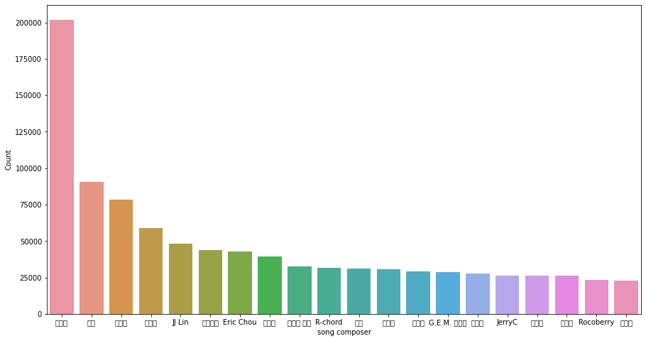
1 2 3 4 5 6 7 8 fig, ax = plt.subplots(1 , figsize=(15 ,8 )) df_composer = user_music_df["composer" ].value_counts().sort_values(ascending=False )[:20 ] ax = sns.barplot([i for i in df_composer.index],df_composer,ax= ax) ax.set_xlabel("song composer" ) ax.set_ylabel("Count" )
Text(0, 0.5, 'Count')
1 df_composer.head(20 ).index
Index(['周杰倫', '阿信', '林俊傑', '陳皓宇', 'JJ Lin', '張簡君偉', 'Eric Chou', '韋禮安',
'八三夭 阿璞', 'R-chord', '怪獸', '吳青峰', '周湯豪', 'G.E.M. 鄧紫棋', '陳小霞', 'JerryC',
'吳克群', '薛之謙', 'Rocoberry', '李榮浩'],
dtype='object')
Analyse the relationship between target and song
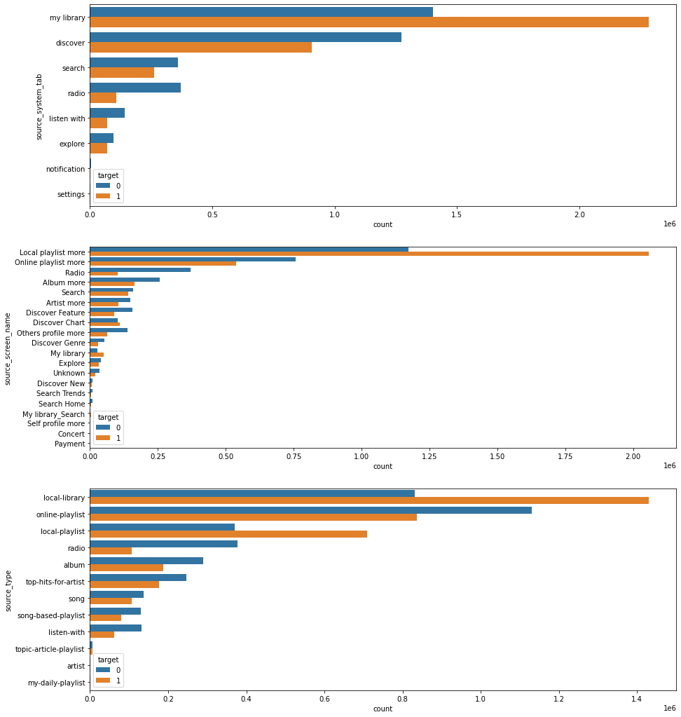
1 2 3 4 5 6 7 8 9 10 11 12 13 14 15 16 17 18 19 20 21 22 23 24 25 26 27 fig, ax = plt.subplots(3 ,1 ,figsize=(15 ,18 )) sns.countplot(y= 'source_system_tab' ,hue='target' , order = user_music_df['source_system_tab' ].value_counts().index, data=user_music_df,dodge=True , ax= ax[0 ]) sns.countplot(y= 'source_screen_name' ,hue='target' , order = user_music_df['source_screen_name' ].value_counts().index, data=user_music_df,dodge=True , ax= ax[1 ]) sns.countplot(y= 'source_type' ,hue='target' , order = user_music_df['source_type' ].value_counts().index, data=user_music_df,dodge=True , ax= ax[2 ])
<matplotlib.axes._subplots.AxesSubplot at 0x7f269a90e128>
We can see that local library and local playlist are the main sources that users repeat playing music and Most of users more prefer to play music from local library than to play music online Analyze Relationship between Target and members info <class 'pandas.core.frame.DataFrame'>
RangeIndex: 34403 entries, 0 to 34402
Data columns (total 7 columns):
# Column Non-Null Count Dtype
--- ------ -------------- -----
0 msno 34403 non-null object
1 city 34403 non-null int64
2 bd 34403 non-null int64
3 gender 14501 non-null object
4 registered_via 34403 non-null int64
5 registration_init_time 34403 non-null int64
6 expiration_date 34403 non-null int64
dtypes: int64(5), object(2)
memory usage: 1.8+ MB
1 2 members_df["registration_init_time" ] = pd.to_datetime(members_df["registration_init_time" ], format="%Y%m%d" ) members_df["expiration_date" ] = pd.to_datetime(members_df["expiration_date" ], format="%Y%m%d" )
Parse the datetime data 1 2 3 4 5 6 7 8 members_df["registration_init_day" ] = members_df["registration_init_time" ].dt.day members_df["registration_init_month" ] = members_df["registration_init_time" ].dt.month members_df["registration_init_year" ] = members_df["registration_init_time" ].dt.year members_df["expiration_day" ] = members_df["expiration_date" ].dt.day members_df["expiration_month" ] = members_df["expiration_date" ].dt.month members_df["expiration_year" ] = members_df["expiration_date" ].dt.year members_df = members_df.drop(columns = ["registration_init_time" , "expiration_date" ],axis=1 ) members_df.info()
<class 'pandas.core.frame.DataFrame'>
RangeIndex: 34403 entries, 0 to 34402
Data columns (total 11 columns):
# Column Non-Null Count Dtype
--- ------ -------------- -----
0 msno 34403 non-null object
1 city 34403 non-null int64
2 bd 34403 non-null int64
3 gender 14501 non-null object
4 registered_via 34403 non-null int64
5 registration_init_day 34403 non-null int64
6 registration_init_month 34403 non-null int64
7 registration_init_year 34403 non-null int64
8 expiration_day 34403 non-null int64
9 expiration_month 34403 non-null int64
10 expiration_year 34403 non-null int64
dtypes: int64(9), object(2)
memory usage: 2.9+ MB
1 2 3 4 5 6 member_music_df = user_music_df.merge(members_df,on='msno' ,how="left" , copy=False ) member_music_df["msno" ] = member_music_df["msno" ].astype("category" ) member_music_df["song_id" ] = member_music_df["song_id" ].astype("category" ) member_music_df.head()
msno
song_id
source_system_tab
source_screen_name
source_type
target
song_length
genre_ids
artist_name
composer
lyricist
language
city
bd
gender
registered_via
registration_init_day
registration_init_month
registration_init_year
expiration_day
expiration_month
expiration_year
0
FGtllVqz18RPiwJj/edr2gV78zirAiY/9SmYvia+kCg=
BBzumQNXUHKdEBOB7mAJuzok+IJA1c2Ryg/yzTF6tik=
explore
Explore
online-playlist
1
206471.0
359
Bastille
Dan Smith| Mark Crew
NaN
52.0
1
0
NaN
7
2
1
2012
5
10
2017
1
Xumu+NIjS6QYVxDS4/t3SawvJ7viT9hPKXmf0RtLNx8=
bhp/MpSNoqoxOIB+/l8WPqu6jldth4DIpCm3ayXnJqM=
my library
Local playlist more
local-playlist
1
284584.0
1259
Various Artists
NaN
NaN
52.0
13
24
female
9
25
5
2011
11
9
2017
2
Xumu+NIjS6QYVxDS4/t3SawvJ7viT9hPKXmf0RtLNx8=
JNWfrrC7zNN7BdMpsISKa4Mw+xVJYNnxXh3/Epw7QgY=
my library
Local playlist more
local-playlist
1
225396.0
1259
Nas
N. Jones、W. Adams、J. Lordan、D. Ingle
NaN
52.0
13
24
female
9
25
5
2011
11
9
2017
3
Xumu+NIjS6QYVxDS4/t3SawvJ7viT9hPKXmf0RtLNx8=
2A87tzfnJTSWqD7gIZHisolhe4DMdzkbd6LzO1KHjNs=
my library
Local playlist more
local-playlist
1
255512.0
1019
Soundway
Kwadwo Donkoh
NaN
-1.0
13
24
female
9
25
5
2011
11
9
2017
4
FGtllVqz18RPiwJj/edr2gV78zirAiY/9SmYvia+kCg=
3qm6XTZ6MOCU11x8FIVbAGH5l5uMkT3/ZalWG1oo2Gc=
explore
Explore
online-playlist
1
187802.0
1011
Brett Young
Brett Young| Kelly Archer| Justin Ebach
NaN
52.0
1
0
NaN
7
2
1
2012
5
10
2017
<class 'pandas.core.frame.DataFrame'>
Int64Index: 7377418 entries, 0 to 7377417
Data columns (total 22 columns):
# Column Dtype
--- ------ -----
0 msno category
1 song_id category
2 source_system_tab object
3 source_screen_name object
4 source_type object
5 target int64
6 song_length float64
7 genre_ids object
8 artist_name object
9 composer object
10 lyricist object
11 language float64
12 city int64
13 bd int64
14 gender object
15 registered_via int64
16 registration_init_day int64
17 registration_init_month int64
18 registration_init_year int64
19 expiration_day int64
20 expiration_month int64
21 expiration_year int64
dtypes: category(2), float64(2), int64(10), object(8)
memory usage: 1.2+ GB
msno 7377418
song_id 7377418
source_system_tab 7352569
source_screen_name 6962614
source_type 7355879
target 7377418
song_length 7377304
genre_ids 7258963
artist_name 7377304
composer 5701712
lyricist 4198620
language 7377268
city 7377418
bd 7377418
gender 4415939
registered_via 7377418
registration_init_day 7377418
registration_init_month 7377418
registration_init_year 7377418
expiration_day 7377418
expiration_month 7377418
expiration_year 7377418
dtype: int64
1 member_music_df['bd' ].describe()
count 7.377418e+06
mean 1.753927e+01
std 2.155447e+01
min -4.300000e+01
25% 0.000000e+00
50% 2.100000e+01
75% 2.900000e+01
max 1.051000e+03
Name: bd, dtype: float64
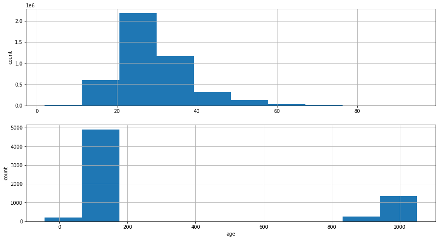
Visualize distribution of age: bd attribution Note: Since this attribute has outliers, I use remove the data that lies outside range [0,100]
1 2 3 4 5 6 7 8 9 fig, ax = plt.subplots(2 , figsize= (15 ,8 )) age_df = member_music_df['bd' ].loc[(member_music_df['bd' ]>0 ) & (member_music_df['bd' ]<100 )] age_df.hist(ax = ax[0 ]) ax[0 ].set_ylabel("count" ) member_music_df['bd' ].loc[(member_music_df['bd' ]<0 ) | (member_music_df['bd' ]>100 )].hist(ax = ax[1 ]) ax[1 ].set_xlabel("age" ) ax[1 ].set_ylabel("count" )
Text(0, 0.5, 'count')
We can see that bd/age has outliers outside range [0,100], so we want to replace the incorrect bd with NaN 1 member_music_df['bd' ].loc[(member_music_df['bd' ]<=0 ) | (member_music_df['bd' ]>=100 )]= np.nan
1 2 member_music_df.describe()
target
song_length
language
city
bd
registered_via
registration_init_day
registration_init_month
registration_init_year
expiration_day
expiration_month
expiration_year
count
7.377418e+06
7.377304e+06
7.377268e+06
7.377418e+06
4.430216e+06
7.377418e+06
7.377418e+06
7.377418e+06
7.377418e+06
7.377418e+06
7.377418e+06
7.377418e+06
mean
5.035171e-01
2.451210e+05
1.860933e+01
7.511399e+00
2.872200e+01
6.794068e+00
1.581532e+01
6.832306e+00
2.012741e+03
1.562338e+01
8.341742e+00
2.017072e+03
std
4.999877e-01
6.734471e+04
2.117681e+01
6.641625e+00
8.634326e+00
2.275774e+00
8.768549e+00
3.700723e+00
3.018861e+00
9.107235e+00
2.511360e+00
3.982536e-01
min
0.000000e+00
1.393000e+03
-1.000000e+00
1.000000e+00
2.000000e+00
3.000000e+00
1.000000e+00
1.000000e+00
2.004000e+03
1.000000e+00
1.000000e+00
1.970000e+03
25%
0.000000e+00
2.147260e+05
3.000000e+00
1.000000e+00
2.300000e+01
4.000000e+00
8.000000e+00
3.000000e+00
2.011000e+03
8.000000e+00
9.000000e+00
2.017000e+03
50%
1.000000e+00
2.418120e+05
3.000000e+00
5.000000e+00
2.700000e+01
7.000000e+00
1.600000e+01
7.000000e+00
2.013000e+03
1.500000e+01
9.000000e+00
2.017000e+03
75%
1.000000e+00
2.721600e+05
5.200000e+01
1.300000e+01
3.300000e+01
9.000000e+00
2.300000e+01
1.000000e+01
2.015000e+03
2.300000e+01
1.000000e+01
2.017000e+03
max
1.000000e+00
1.085171e+07
5.900000e+01
2.200000e+01
9.500000e+01
1.300000e+01
3.100000e+01
1.200000e+01
2.017000e+03
3.100000e+01
1.200000e+01
2.020000e+03
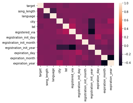
1 2 3 4 corr_matrix = member_music_df.corr() _ = sns.heatmap(corr_matrix)
1 2 3 4 5 6 7 8 9 10 11 12 13 14 15 16 17 18 19 20 21 22 23 24 25 26 27 28 29 30 31 32 33 34 35 36 37 38 39 40 41 42 43 44 45 46 47 48 49 50 51 52 53 54 corr = corr_matrix['target' ].sort_values(ascending= False ) for x in corr.index[1 :4 ].to_list(): print("{} {}" .format(x, corr[x])) print("" ) corr = corr_matrix['song_length' ].sort_values(ascending= False ) for x in corr.index[1 :4 ].to_list(): print("{} {}" .format(x, corr[x])) print("" ) corr = corr_matrix['language' ].sort_values(ascending= False ) for x in corr.index[1 :4 ].to_list(): print("{} {}" .format(x, corr[x])) print("" ) corr = corr_matrix['city' ].sort_values(ascending= False ) for x in corr.index[1 :4 ].to_list(): print("{} {}" .format(x, corr[x])) print("" ) corr = corr_matrix['bd' ].sort_values(ascending= False ) for x in corr.index[1 :4 ].to_list(): print("{} {}" .format(x, corr[x])) print("" ) corr = corr_matrix['registered_via' ].sort_values(ascending= False ) for x in corr.index[1 :4 ].to_list(): print("{} {}" .format(x, corr[x])) print("" ) corr = corr_matrix['registration_init_day' ].sort_values(ascending= False ) for x in corr.index[1 :4 ].to_list(): print("{} {}" .format(x, corr[x])) print("" ) corr = corr_matrix['registration_init_month' ].sort_values(ascending= False ) for x in corr.index[1 :4 ].to_list(): print("{} {}" .format(x, corr[x])) print("" ) corr = corr_matrix['registration_init_year' ].sort_values(ascending= False ) for x in corr.index[1 :4 ].to_list(): print("{} {}" .format(x, corr[x])) print("" ) corr = corr_matrix['expiration_day' ].sort_values(ascending= False ) for x in corr.index[1 :4 ].to_list(): print("{} {}" .format(x, corr[x])) print("" ) corr = corr_matrix['expiration_month' ].sort_values(ascending= False ) for x in corr.index[1 :4 ].to_list(): print("{} {}" .format(x, corr[x])) print("" ) corr = corr_matrix['expiration_year' ].sort_values(ascending= False ) for x in corr.index[1 :4 ].to_list(): print("{} {}" .format(x, corr[x])) print("" )
expiration_year 0.042248332355979766
city 0.01211438566189457
expiration_month 0.011817072086387569
bd 0.009861302779254176
city 0.005184912771179072
expiration_year 0.00457185870016758
registration_init_year 0.009070490482763404
registration_init_day 0.001510510575428178
bd 0.001107978394135987
expiration_year 0.15014690465127595
registered_via 0.0737556175747622
target 0.01211438566189457
registered_via 0.1753390015877422
expiration_day 0.056335854806629254
expiration_month 0.032935904360496926
bd 0.1753390015877422
expiration_year 0.08413460079453493
city 0.0737556175747622
expiration_day 0.1493505099924221
registration_init_month 0.04443692475737983
registered_via 0.02554331305533987
expiration_month 0.056911114419175665
registration_init_day 0.04443692475737983
bd 0.005399463812914416
language 0.009070490482763404
target -0.00196242388069252
song_length -0.007434856516605977
registration_init_day 0.1493505099924221
registered_via 0.05695618668075027
bd 0.056335854806629254
registered_via 0.0647318000666518
registration_init_month 0.056911114419175665
bd 0.032935904360496926
city 0.15014690465127595
registered_via 0.08413460079453493
target 0.042248332355979766
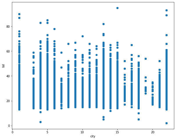
1 2 3 4 5 6 fig, ax = plt.subplots(1 ,1 ,figsize=(10 ,8 ), sharex=False ) plt.scatter(x = member_music_df['city' ],y = member_music_df['bd' ]) ax.set_ylabel("bd" ) ax.set_xlabel("city" ) plt.show()
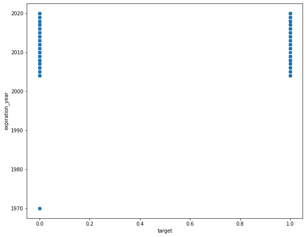
1 2 3 4 5 6 fig, ax = plt.subplots(1 ,1 ,figsize=(10 ,8 ), sharex=False ) plt.scatter(x = member_music_df['target' ],y = member_music_df['expiration_year' ]) ax.set_ylabel("expiration_year" ) ax.set_xlabel("target" ) plt.show()
1 2 3 4 5 print(train_df.target.value_counts()*100 /train_df.target.value_counts().sum()) print('unique songs ' ,len(train_df.song_id.unique()))
1 50.351708
0 49.648292
Name: target, dtype: float64
unique songs 359966
1 2 3 4 5 6 7 repeats=train_df[train_df.target==1 ] song_repeats=repeats.groupby('song_id' ,as_index=False ).msno.count() song_repeats.columns=['song_id' ,'count' ] song_repeats=pd.DataFrame(song_repeats).merge(song_df,left_on='song_id' ,right_on='song_id' ) print("Print top 50 songs repeated" ) repeats.song_id.value_counts().head(50 )
Print top 50 songs repeated
reXuGcEWDDCnL0K3Th//3DFG4S1ACSpJMzA+CFipo1g= 10885
T86YHdD4C9JSc274b1IlMkLuNdz4BQRB50fWWE7hx9g= 10556
FynUyq0+drmIARmK1JZ/qcjNZ7DKkqTY6/0O0lTzNUI= 9808
wBTWuHbjdjxnG1lQcbqnK4FddV24rUhuyrYLd9c/hmk= 9411
PgRtmmESVNtWjoZHO5a1r21vIz9sVZmcJJpFCbRa1LI= 9004
U9kojfZSKaiWOW94PKh1Riyv/zUWxmBRmv0XInQWLGw= 8787
YN4T/yvvXtYrBVN8KTnieiQohHL3T9fnzUkbLWcgLro= 8780
M9rAajz4dYuRhZ7jLvf9RRayVA3os61X/XXHEuW4giA= 8403
43Qm2YzsP99P5wm37B1JIhezUcQ/1CDjYlQx6rBbz2U= 8112
J4qKkLIoW7aYACuTupHLAPZYmRp08en1AEux+GSUzdw= 7903
cy10N2j2sdY/X4BDUcMu2Iumfz7pV3tqE5iEaup2yGI= 7725
750RprmFfLV0bymtDH88g24pLZGVi5VpBAI300P6UOA= 7608
IKMFuL0f5Y8c63Hg9BXkeNJjE0z8yf3gMt/tOxF4QNE= 7224
+SstqMwhQPBQFTPBhLKPT642IiBDXzZFwlzsLl4cGXo= 7061
DLBDZhOoW7zd7GBV99bi92ZXYUS26lzV+jJKbHshP5c= 6901
v/3onppBGoSpGsWb8iaCIO8eX5+iacbH5a4ZUhT7N54= 6879
p/yR06j/RQ2J6yGCFL0K+1R06OeG+eXcwxRgOHDo/Tk= 6536
Xpjwi8UAE2Vv9PZ6cZnhc58MCtl3cKZEO1sdAkqJ4mo= 6399
OaEbZ6TJ1NePtNUeEgWsvFLeopkSln9WQu8PBR5B3+A= 6187
BITuBuNyXQydJcjDL2BUnCu4/IXaJg5IPOuycc/4dtY= 6160
BgqjNqzsyCpEGvxyUmktvHC8WO5+FQO/pQTaZ4broMU= 6140
3VkD5ekIf5duJm1hmYTZlXjyl0zqV8wCzuAh3uocfCg= 6012
8Ckw1wek5d6oEsNUoM4P5iag86TaEmyLwdtrckL0Re8= 6003
n+pMhj/jpCnpiUcSDl4k3i9FJODDddEXmpE48/HczTI= 5787
WL4ipO3Mx9pxd4FMs69ha6o9541+fLeOow67Qkrfnro= 5784
/70HjygVDhHsKBoV8mmsBg/WduSgs4+Zg6GfzhUQbdk= 5588
L6w2d0w84FjTvFr+BhMfgu7dZAsGiOqUGmvvxIG3gvQ= 5480
fEAIgFRWmhXmo6m3ukQeqRksZCcO/7CjkqNckRHiVQo= 5460
+Sm75wnBf/sjm/QMUAFx8N+Ae04kWCXGlgH50tTeM6c= 5412
VkDBgh89umc9m6uAEfD6LXngetyGhln4vh/ArCGO0nY= 5361
fCCmIa0Y5m+MCGbQga31MOLTIqi7ddgXvkjFPmfslGw= 5305
+LztcJcPEEwsikk6+K5udm06XJQMzR4+lzavKLUyE0k= 5298
o9HWMBZMeIPnYEpSuscGoORKE44sj3BYOdvGuIi0P68= 5233
QZBm8SOwnEjNfCpgsKBBGPMGET6y6XaQgnJiirspW7I= 5224
ClazTFnk6r0Bnuie44bocdNMM3rdlrq0bCGAsGUWcHE= 5202
wp1gSQ4LlMEF6bzvEaJl8VdHlAj/EJMTJ0ASrXeddbo= 5110
THqGcrzQyUhBn1NI/+Iptc1vKtxBIEg0uA8iaoJnO1Q= 5086
ys+EL8Sok4HC4i7sDY0+slDNGVZ8+uOQi6TQ6g8VSF4= 5012
zHqZ07gn+YvF36FWzv9+y8KiCMhYhdAUS+vSIKY3UZY= 5001
8f/T4ohROj1wa25YHMItOW2/wJhRXZM0+T5/2p86COc= 4982
G/4+VCRLpfjQJ4SAwMDcf+W8PTw0eOBRgFvg4fHUOO8= 4956
KZ5hwP74wRO6kRapVIprwodtNdVD2EVD3hkZmmyXFPk= 4888
MtFK4NN8Kv1k/xPA3wb8SQaP/jWee52FAaC1s9NFsU4= 4813
UQeOwfhcqgEcIwp3cgNiLGW1237Qjpvqzt/asQimVp0= 4778
JA6C0GEK1sSCVbHyqtruH/ARD1NKolYrw7HXy6EVNAc= 4766
8qWeDv6RTv+hYJxW94e7n6HBzHPGPEZW9FuGhj6pPhQ= 4761
35dx60z4m4+Lg+qIS0l2A8vspbthqnpTylWUu51jW+4= 4679
r4lUPUkz3tAgIWaEyrSYVCxX1yz8PnlVuQz+To0Pd+c= 4650
1PR/lVwL4VeYcZjexwBJ2NOSTfgh8JoVxWCunnbJO/8= 4592
7EnDBkQYJpipCyRd9JBsug4iKnfAunUXc14/96cNotg= 4571
Name: song_id, dtype: int64
2. Data Preprocessing Note: This section is to show how to preprocess data. We can also directly start from Step 3 for data extract, transformation and load using integrated transformation function and skip this step if necessary
2.1 Filling missing values 1 2 missing_value_cols = [c for c in member_music_df.columns if member_music_df[c].isnull().any()] missing_value_cols
['source_system_tab',
'source_screen_name',
'source_type',
'song_length',
'genre_ids',
'artist_name',
'composer',
'lyricist',
'language',
'bd',
'gender']
msno 7377418
song_id 7377418
source_system_tab 7352569
source_screen_name 6962614
source_type 7355879
target 7377418
song_length 7377304
genre_ids 7258963
artist_name 7377304
composer 5701712
lyricist 4198620
language 7377268
city 7377418
bd 4430216
gender 4415939
registered_via 7377418
registration_init_day 7377418
registration_init_month 7377418
registration_init_year 7377418
expiration_day 7377418
expiration_month 7377418
expiration_year 7377418
dtype: int64
1 2 3 4 5 6 7 8 9 10 11 12 13 14 15 16 17 18 19 20 21 22 23 24 25 26 27 28 29 def fill_missing_value_v1 (x) : return x.fillna(x.value_counts().sort_values(ascending=False ).index[0 ]) categorical_ls = ['source_system_tab' , 'source_screen_name' ,'source_type' ,'genre_ids' ,'artist_name' ,'composer' , 'lyricist' ,'gender' ] numerical_ls = ['song_length' ,'language' ,'bd' ] for index in numerical_ls: member_music_df[index].fillna(member_music_df[index].median(), inplace=True ) for index in categorical_ls: member_music_df[index].fillna("no_data" , inplace=True )
msno 7377418
song_id 7377418
source_system_tab 7377418
source_screen_name 7377418
source_type 7377418
target 7377418
song_length 7377418
genre_ids 7377418
artist_name 7377418
composer 7377418
lyricist 7377418
language 7377418
city 7377418
bd 7377418
gender 7377418
registered_via 7377418
registration_init_day 7377418
registration_init_month 7377418
registration_init_year 7377418
expiration_day 7377418
expiration_month 7377418
expiration_year 7377418
dtype: int64
1 2 member_music_df[numerical_ls].head(100 )
song_length
language
bd
0
206471.0
52.0
27.0
1
284584.0
52.0
24.0
2
225396.0
52.0
24.0
3
255512.0
-1.0
24.0
4
187802.0
52.0
27.0
...
...
...
...
95
333024.0
3.0
27.0
96
288391.0
3.0
46.0
97
279196.0
3.0
46.0
98
240744.0
3.0
46.0
99
221622.0
3.0
46.0
100 rows × 3 columns
1 2 member_music_df[categorical_ls].head(100 )
source_system_tab
source_screen_name
source_type
genre_ids
artist_name
composer
lyricist
gender
0
explore
Explore
online-playlist
359
Bastille
Dan Smith| Mark Crew
no_data
no_data
1
my library
Local playlist more
local-playlist
1259
Various Artists
no_data
no_data
female
2
my library
Local playlist more
local-playlist
1259
Nas
N. Jones、W. Adams、J. Lordan、D. Ingle
no_data
female
3
my library
Local playlist more
local-playlist
1019
Soundway
Kwadwo Donkoh
no_data
female
4
explore
Explore
online-playlist
1011
Brett Young
Brett Young| Kelly Archer| Justin Ebach
no_data
no_data
...
...
...
...
...
...
...
...
...
95
my library
no_data
local-library
458
楊乃文 (Naiwen Yang)
黃建為
葛大為
male
96
my library
Local playlist more
local-library
458
陳奕迅 (Eason Chan)
Jun Jie Lin
no_data
female
97
my library
Local playlist more
local-library
458
周杰倫 (Jay Chou)
周杰倫
方文山
female
98
my library
Local playlist more
local-library
465
范瑋琪 (Christine Fan)
非非
非非
female
99
my library
Local playlist more
local-library
465|1259
玖壹壹
陳皓宇
廖建至|洪瑜鴻
female
100 rows × 8 columns
We can see that the columns like genre_ids, composer, lyricist have multiple values in a cell. In this case, the count of genres, composers, lyricist could be useful information as well
Index(['msno', 'song_id', 'source_system_tab', 'source_screen_name',
'source_type', 'target', 'song_length', 'genre_ids', 'artist_name',
'composer', 'lyricist', 'language', 'city', 'bd', 'gender',
'registered_via', 'registration_init_day', 'registration_init_month',
'registration_init_year', 'expiration_day', 'expiration_month',
'expiration_year'],
dtype='object')
1 member_music_df.genre_ids.nunique(), member_music_df.composer.nunique(), member_music_df.lyricist.nunique()
(573, 76065, 33889)
1 2 3 4 5 6 7 8 9 def count_items (x) : if x =="no_data" : return 0 return sum(map(x.count, ['|' , '/' , '\\' , ';' ,',' ])) + 1 member_music_df['genre_count' ]= member_music_df['genre_ids' ].apply(count_items) member_music_df['composer_count' ]= member_music_df['composer' ].apply(count_items) member_music_df['lyricist_count' ]= member_music_df['lyricist' ].apply(count_items)
msno
song_id
source_system_tab
source_screen_name
source_type
target
song_length
genre_ids
artist_name
composer
lyricist
language
city
bd
gender
registered_via
registration_init_day
registration_init_month
registration_init_year
expiration_day
expiration_month
expiration_year
genre_count
composer_count
lyricist_count
0
FGtllVqz18RPiwJj/edr2gV78zirAiY/9SmYvia+kCg=
BBzumQNXUHKdEBOB7mAJuzok+IJA1c2Ryg/yzTF6tik=
explore
Explore
online-playlist
1
206471.0
359
Bastille
Dan Smith| Mark Crew
no_data
52.0
1
27.0
no_data
7
2
1
2012
5
10
2017
1
2
0
1
Xumu+NIjS6QYVxDS4/t3SawvJ7viT9hPKXmf0RtLNx8=
bhp/MpSNoqoxOIB+/l8WPqu6jldth4DIpCm3ayXnJqM=
my library
Local playlist more
local-playlist
1
284584.0
1259
Various Artists
no_data
no_data
52.0
13
24.0
female
9
25
5
2011
11
9
2017
1
0
0
2
Xumu+NIjS6QYVxDS4/t3SawvJ7viT9hPKXmf0RtLNx8=
JNWfrrC7zNN7BdMpsISKa4Mw+xVJYNnxXh3/Epw7QgY=
my library
Local playlist more
local-playlist
1
225396.0
1259
Nas
N. Jones、W. Adams、J. Lordan、D. Ingle
no_data
52.0
13
24.0
female
9
25
5
2011
11
9
2017
1
1
0
3
Xumu+NIjS6QYVxDS4/t3SawvJ7viT9hPKXmf0RtLNx8=
2A87tzfnJTSWqD7gIZHisolhe4DMdzkbd6LzO1KHjNs=
my library
Local playlist more
local-playlist
1
255512.0
1019
Soundway
Kwadwo Donkoh
no_data
-1.0
13
24.0
female
9
25
5
2011
11
9
2017
1
1
0
4
FGtllVqz18RPiwJj/edr2gV78zirAiY/9SmYvia+kCg=
3qm6XTZ6MOCU11x8FIVbAGH5l5uMkT3/ZalWG1oo2Gc=
explore
Explore
online-playlist
1
187802.0
1011
Brett Young
Brett Young| Kelly Archer| Justin Ebach
no_data
52.0
1
27.0
no_data
7
2
1
2012
5
10
2017
1
3
0
We can skip Step 2 if we just want to transform data directly
1 2 3 4 5 6 7 8 9 10 11 12 import warningswarnings.filterwarnings('ignore' ) import numpy as np import pandas as pdimport matplotlib.pyplot as pltimport seaborn as snsimport lightgbm as lgbfrom subprocess import check_outputnp.random.seed(2020 )
1 2 3 4 5 6 7 8 9 10 11 12 13 14 15 16 17 18 19 20 21 22 23 24 25 26 27 28 29 30 31 32 33 34 35 36 37 38 39 40 41 42 43 44 45 46 47 48 49 50 51 52 def transform_data (data, song_df, members_df) : data = data.merge(song_df,on='song_id' ,how="left" , copy =False ) members_df["registration_init_time" ] = pd.to_datetime(members_df["registration_init_time" ], format="%Y%m%d" ) members_df["expiration_date" ] = pd.to_datetime(members_df["expiration_date" ], format="%Y%m%d" ) members_df["registration_init_day" ] = members_df["registration_init_time" ].dt.day members_df["registration_init_month" ] = members_df["registration_init_time" ].dt.month members_df["registration_init_year" ] = members_df["registration_init_time" ].dt.year members_df["expiration_day" ] = members_df["expiration_date" ].dt.day members_df["expiration_month" ] = members_df["expiration_date" ].dt.month members_df["expiration_year" ] = members_df["expiration_date" ].dt.year members_df = members_df.drop(columns = ["registration_init_time" , "expiration_date" ],axis=1 ) data = data.merge(members_df,on='msno' ,how="left" , copy=False ) data['bd' ].loc[(data['bd' ]<=0 ) | (data['bd' ]>=100 )]= np.nan categorical_ls = ['source_system_tab' , 'source_screen_name' ,'source_type' ,'genre_ids' ,'artist_name' ,'composer' , 'lyricist' ,'gender' ] numerical_ls = ['song_length' ,'language' ,'bd' ] for index in numerical_ls: data[index].fillna(data[index].median(), inplace=True ) for index in categorical_ls: data[index].fillna("no_data" , inplace=True ) def count_items (x) : if x =="no_data" : return 0 return sum(map(x.count, ['|' , '/' , '\\' , ';' ,',' ])) + 1 data['genre_count' ]= data['genre_ids' ].apply(count_items) data['composer_count' ]= data['composer' ].apply(count_items) data['lyricist_count' ]= data['lyricist' ].apply(count_items) for c in data.columns: if data[c].dtype=='O' : data[c] = data[c].astype("category" ,copy=False ) if 'id' in data.columns: ids = data['id' ] data.drop(['id' ], inplace=True ,axis=1 ) else : ids =None return ids, data
1 2 3 4 5 6 root = './kaggle/working/train/data/' train_df = pd.read_csv(root+ "train.csv" ) test_df = pd.read_csv(root+ "test.csv" ) song_df = pd.read_csv(root+ "songs.csv" ) members_df = pd.read_csv(root+ "members.csv" )
1 _, train_data = transform_data(train_df, song_df, members_df)
1 2 3 y_train = train_data['target' ] train_data.drop(['target' ], axis=1 ,inplace=True ) X_train = train_data
Transform the name of composer, artist, lyricist to new features like counts, number of intersection of names
1 2 3 4 5 6 7 8 9 10 11 12 13 14 15 16 def transform_names_intersection (data) : def check_name_list (x) : strings = None strings = x.str.split(r"//|/|;|、|\| " ) return strings df = data[["composer" ,"artist_name" , "lyricist" ]].apply(check_name_list) data["composer_artist_intersect" ] =[len(set(a) & set(b)) for a, b in zip(df.composer, df.artist_name)] data["composer_lyricist_intersect" ] =[len(set(a) & set(b)) for a, b in zip(df.composer, df.lyricist)] data["artist_lyricist_intersect" ] =[len(set(a) & set(b)) for a, b in zip(df.artist_name, df.lyricist)] return data _ = transform_names_intersection(X_train) X_train.head()
msno
song_id
source_system_tab
source_screen_name
source_type
song_length
genre_ids
artist_name
composer
lyricist
language
city
bd
gender
registered_via
registration_init_day
registration_init_month
registration_init_year
expiration_day
expiration_month
expiration_year
genre_count
composer_count
lyricist_count
composer_artist_intersect
composer_lyricist_intersect
artist_lyricist_intersect
0
FGtllVqz18RPiwJj/edr2gV78zirAiY/9SmYvia+kCg=
BBzumQNXUHKdEBOB7mAJuzok+IJA1c2Ryg/yzTF6tik=
explore
Explore
online-playlist
206471.0
359
Bastille
Dan Smith| Mark Crew
no_data
52.0
1
27.0
no_data
7
2
1
2012
5
10
2017
1
2
0
0
0
0
1
Xumu+NIjS6QYVxDS4/t3SawvJ7viT9hPKXmf0RtLNx8=
bhp/MpSNoqoxOIB+/l8WPqu6jldth4DIpCm3ayXnJqM=
my library
Local playlist more
local-playlist
284584.0
1259
Various Artists
no_data
no_data
52.0
13
24.0
female
9
25
5
2011
11
9
2017
1
0
0
0
1
0
2
Xumu+NIjS6QYVxDS4/t3SawvJ7viT9hPKXmf0RtLNx8=
JNWfrrC7zNN7BdMpsISKa4Mw+xVJYNnxXh3/Epw7QgY=
my library
Local playlist more
local-playlist
225396.0
1259
Nas
N. Jones、W. Adams、J. Lordan、D. Ingle
no_data
52.0
13
24.0
female
9
25
5
2011
11
9
2017
1
1
0
0
0
0
3
Xumu+NIjS6QYVxDS4/t3SawvJ7viT9hPKXmf0RtLNx8=
2A87tzfnJTSWqD7gIZHisolhe4DMdzkbd6LzO1KHjNs=
my library
Local playlist more
local-playlist
255512.0
1019
Soundway
Kwadwo Donkoh
no_data
-1.0
13
24.0
female
9
25
5
2011
11
9
2017
1
1
0
0
0
0
4
FGtllVqz18RPiwJj/edr2gV78zirAiY/9SmYvia+kCg=
3qm6XTZ6MOCU11x8FIVbAGH5l5uMkT3/ZalWG1oo2Gc=
explore
Explore
online-playlist
187802.0
1011
Brett Young
Brett Young| Kelly Archer| Justin Ebach
no_data
52.0
1
27.0
no_data
7
2
1
2012
5
10
2017
1
3
0
1
0
0
1 2 3 ids, test_data = transform_data(test_df, song_df, members_df) _ = transform_names_intersection(test_data) test_data.head()
msno
song_id
source_system_tab
source_screen_name
source_type
song_length
genre_ids
artist_name
composer
lyricist
language
city
bd
gender
registered_via
registration_init_day
registration_init_month
registration_init_year
expiration_day
expiration_month
expiration_year
genre_count
composer_count
lyricist_count
composer_artist_intersect
composer_lyricist_intersect
artist_lyricist_intersect
0
V8ruy7SGk7tDm3zA51DPpn6qutt+vmKMBKa21dp54uM=
WmHKgKMlp1lQMecNdNvDMkvIycZYHnFwDT72I5sIssc=
my library
Local playlist more
local-library
224130.0
458
梁文音 (Rachel Liang)
Qi Zheng Zhang
no_data
3.0
1
27.0
no_data
7
19
2
2016
18
9
2017
1
1
0
0
0
0
1
V8ruy7SGk7tDm3zA51DPpn6qutt+vmKMBKa21dp54uM=
y/rsZ9DC7FwK5F2PK2D5mj+aOBUJAjuu3dZ14NgE0vM=
my library
Local playlist more
local-library
320470.0
465
林俊傑 (JJ Lin)
林俊傑
孫燕姿/易家揚
3.0
1
27.0
no_data
7
19
2
2016
18
9
2017
1
1
2
0
0
0
2
/uQAlrAkaczV+nWCd2sPF2ekvXPRipV7q0l+gbLuxjw=
8eZLFOdGVdXBSqoAv5nsLigeH2BvKXzTQYtUM53I0k4=
discover
no_data
song-based-playlist
315899.0
2022
Yu Takahashi (高橋優)
Yu Takahashi
Yu Takahashi
17.0
1
27.0
no_data
4
17
11
2016
24
11
2016
1
1
1
0
1
0
3
1a6oo/iXKatxQx4eS9zTVD+KlSVaAFbTIqVvwLC1Y0k=
ztCf8thYsS4YN3GcIL/bvoxLm/T5mYBVKOO4C9NiVfQ=
radio
Radio
radio
285210.0
465
U2
The Edge| Adam Clayton| Larry Mullen| Jr.
no_data
52.0
3
30.0
male
9
25
7
2007
30
4
2017
1
4
0
0
0
0
4
1a6oo/iXKatxQx4eS9zTVD+KlSVaAFbTIqVvwLC1Y0k=
MKVMpslKcQhMaFEgcEQhEfi5+RZhMYlU3eRDpySrH8Y=
radio
Radio
radio
197590.0
873
Yoga Mr Sound
Neuromancer
no_data
-1.0
3
30.0
male
9
25
7
2007
30
4
2017
1
1
0
0
0
0
msno
song_id
source_system_tab
source_screen_name
source_type
song_length
genre_ids
artist_name
composer
lyricist
language
city
bd
gender
registered_via
registration_init_day
registration_init_month
registration_init_year
expiration_day
expiration_month
expiration_year
genre_count
composer_count
lyricist_count
composer_artist_intersect
composer_lyricist_intersect
artist_lyricist_intersect
0
FGtllVqz18RPiwJj/edr2gV78zirAiY/9SmYvia+kCg=
BBzumQNXUHKdEBOB7mAJuzok+IJA1c2Ryg/yzTF6tik=
explore
Explore
online-playlist
206471.0
359
Bastille
Dan Smith| Mark Crew
no_data
52.0
1
27.0
no_data
7
2
1
2012
5
10
2017
1
2
0
0
0
0
1
Xumu+NIjS6QYVxDS4/t3SawvJ7viT9hPKXmf0RtLNx8=
bhp/MpSNoqoxOIB+/l8WPqu6jldth4DIpCm3ayXnJqM=
my library
Local playlist more
local-playlist
284584.0
1259
Various Artists
no_data
no_data
52.0
13
24.0
female
9
25
5
2011
11
9
2017
1
0
0
0
1
0
2
Xumu+NIjS6QYVxDS4/t3SawvJ7viT9hPKXmf0RtLNx8=
JNWfrrC7zNN7BdMpsISKa4Mw+xVJYNnxXh3/Epw7QgY=
my library
Local playlist more
local-playlist
225396.0
1259
Nas
N. Jones、W. Adams、J. Lordan、D. Ingle
no_data
52.0
13
24.0
female
9
25
5
2011
11
9
2017
1
1
0
0
0
0
3
Xumu+NIjS6QYVxDS4/t3SawvJ7viT9hPKXmf0RtLNx8=
2A87tzfnJTSWqD7gIZHisolhe4DMdzkbd6LzO1KHjNs=
my library
Local playlist more
local-playlist
255512.0
1019
Soundway
Kwadwo Donkoh
no_data
-1.0
13
24.0
female
9
25
5
2011
11
9
2017
1
1
0
0
0
0
4
FGtllVqz18RPiwJj/edr2gV78zirAiY/9SmYvia+kCg=
3qm6XTZ6MOCU11x8FIVbAGH5l5uMkT3/ZalWG1oo2Gc=
explore
Explore
online-playlist
187802.0
1011
Brett Young
Brett Young| Kelly Archer| Justin Ebach
no_data
52.0
1
27.0
no_data
7
2
1
2012
5
10
2017
1
3
0
1
0
0
msno
song_id
source_system_tab
source_screen_name
source_type
song_length
genre_ids
artist_name
composer
lyricist
language
city
bd
gender
registered_via
registration_init_day
registration_init_month
registration_init_year
expiration_day
expiration_month
expiration_year
genre_count
composer_count
lyricist_count
composer_artist_intersect
composer_lyricist_intersect
artist_lyricist_intersect
0
V8ruy7SGk7tDm3zA51DPpn6qutt+vmKMBKa21dp54uM=
WmHKgKMlp1lQMecNdNvDMkvIycZYHnFwDT72I5sIssc=
my library
Local playlist more
local-library
224130.0
458
梁文音 (Rachel Liang)
Qi Zheng Zhang
no_data
3.0
1
27.0
no_data
7
19
2
2016
18
9
2017
1
1
0
0
0
0
1
V8ruy7SGk7tDm3zA51DPpn6qutt+vmKMBKa21dp54uM=
y/rsZ9DC7FwK5F2PK2D5mj+aOBUJAjuu3dZ14NgE0vM=
my library
Local playlist more
local-library
320470.0
465
林俊傑 (JJ Lin)
林俊傑
孫燕姿/易家揚
3.0
1
27.0
no_data
7
19
2
2016
18
9
2017
1
1
2
0
0
0
2
/uQAlrAkaczV+nWCd2sPF2ekvXPRipV7q0l+gbLuxjw=
8eZLFOdGVdXBSqoAv5nsLigeH2BvKXzTQYtUM53I0k4=
discover
no_data
song-based-playlist
315899.0
2022
Yu Takahashi (高橋優)
Yu Takahashi
Yu Takahashi
17.0
1
27.0
no_data
4
17
11
2016
24
11
2016
1
1
1
0
1
0
3
1a6oo/iXKatxQx4eS9zTVD+KlSVaAFbTIqVvwLC1Y0k=
ztCf8thYsS4YN3GcIL/bvoxLm/T5mYBVKOO4C9NiVfQ=
radio
Radio
radio
285210.0
465
U2
The Edge| Adam Clayton| Larry Mullen| Jr.
no_data
52.0
3
30.0
male
9
25
7
2007
30
4
2017
1
4
0
0
0
0
4
1a6oo/iXKatxQx4eS9zTVD+KlSVaAFbTIqVvwLC1Y0k=
MKVMpslKcQhMaFEgcEQhEfi5+RZhMYlU3eRDpySrH8Y=
radio
Radio
radio
197590.0
873
Yoga Mr Sound
Neuromancer
no_data
-1.0
3
30.0
male
9
25
7
2007
30
4
2017
1
1
0
0
0
0
3.2.3 Split validation set and trainset 1 2 3 4 5 6 7 8 9 from sklearn.model_selection import StratifiedShuffleSplit, StratifiedKFold, train_test_splitss_split = StratifiedShuffleSplit(n_splits=1 , test_size=0.2 , random_state=2021 ) train_index, valid_index ,test_index = None , None , None for train_i, test_i in ss_split.split(np.zeros(y_train.shape) ,y_train): train_index = train_i test_index = test_i print(train_index.shape, test_index.shape)
(5901934,) (1475484,)
1 2 3 4 5 6 7 8 X_validset = X_train.iloc[test_index] y_validset = y_train.iloc[test_index].values X_trainset = X_train.iloc[train_index] y_trainset = y_train.iloc[train_index].values del X_train, y_train
<class 'pandas.core.frame.DataFrame'>
Int64Index: 5901934 entries, 7066318 to 5275539
Data columns (total 27 columns):
# Column Dtype
--- ------ -----
0 msno category
1 song_id category
2 source_system_tab category
3 source_screen_name category
4 source_type category
5 song_length float64
6 genre_ids category
7 artist_name category
8 composer category
9 lyricist category
10 language float64
11 city int64
12 bd float64
13 gender category
14 registered_via int64
15 registration_init_day int64
16 registration_init_month int64
17 registration_init_year int64
18 expiration_day int64
19 expiration_month int64
20 expiration_year int64
21 genre_count int64
22 composer_count int64
23 lyricist_count int64
24 composer_artist_intersect int64
25 composer_lyricist_intersect int64
26 artist_lyricist_intersect int64
dtypes: category(10), float64(3), int64(14)
memory usage: 966.0 MB
4. LGBM Modeling 1 2 3 import lightgbm as lgbtrain_set = lgb.Dataset(X_trainset, y_trainset) valid_set = lgb.Dataset(X_validset, y_validset)
1 2 num_leaves = 110 max_depths = [10 , 15 , 20 , 25 ,30 ]
5.Model Training and Validation on LGBM models 1 2 3 4 5 6 7 8 9 10 11 12 13 14 15 16 17 18 19 params = { 'objective' : 'binary' , 'metric' : 'binary_logloss' , 'boosting' : 'gbdt' , 'learning_rate' : 0.3 , 'verbose' : 0 , 'num_leaves' : num_leaves, 'bagging_fraction' : 0.95 , 'bagging_freq' : 1 , 'bagging_seed' : 1 , 'feature_fraction' : 0.9 , 'feature_fraction_seed' : 1 , 'max_bin' : 256 , 'max_depth' : max_depths[0 ], 'num_rounds' : 200 , 'metric' : 'auc' } %time model_f1 = lgb.train(params, train_set=train_set, valid_sets=valid_set, verbose_eval=5 )
[5] valid_0's auc: 0.710928
[10] valid_0's auc: 0.723954
[15] valid_0's auc: 0.731661
[20] valid_0's auc: 0.736653
[25] valid_0's auc: 0.740424
[30] valid_0's auc: 0.744678
[35] valid_0's auc: 0.749056
[40] valid_0's auc: 0.752277
[45] valid_0's auc: 0.754501
[50] valid_0's auc: 0.756448
[55] valid_0's auc: 0.758097
[60] valid_0's auc: 0.75991
[65] valid_0's auc: 0.761418
[70] valid_0's auc: 0.762683
[75] valid_0's auc: 0.764243
[80] valid_0's auc: 0.765646
[85] valid_0's auc: 0.766883
[90] valid_0's auc: 0.767921
[95] valid_0's auc: 0.769111
[100] valid_0's auc: 0.770006
[105] valid_0's auc: 0.770934
[110] valid_0's auc: 0.772012
[115] valid_0's auc: 0.772747
[120] valid_0's auc: 0.773835
[125] valid_0's auc: 0.774486
[130] valid_0's auc: 0.775258
[135] valid_0's auc: 0.775887
[140] valid_0's auc: 0.776838
[145] valid_0's auc: 0.777587
[150] valid_0's auc: 0.778113
[155] valid_0's auc: 0.778714
[160] valid_0's auc: 0.77929
[165] valid_0's auc: 0.779884
[170] valid_0's auc: 0.780354
[175] valid_0's auc: 0.781586
[180] valid_0's auc: 0.782002
[185] valid_0's auc: 0.782517
[190] valid_0's auc: 0.783075
[195] valid_0's auc: 0.783496
[200] valid_0's auc: 0.784083
CPU times: user 8min 20s, sys: 3 s, total: 8min 23s
Wall time: 4min 25s
1 2 3 4 5 6 7 8 9 10 11 12 13 14 15 16 17 18 19 params = { 'objective' : 'binary' , 'metric' : 'binary_logloss' , 'boosting' : 'gbdt' , 'learning_rate' : 0.3 , 'verbose' : 0 , 'num_leaves' : num_leaves, 'bagging_fraction' : 0.95 , 'bagging_freq' : 1 , 'bagging_seed' : 1 , 'feature_fraction' : 0.9 , 'feature_fraction_seed' : 1 , 'max_bin' : 256 , 'max_depth' : max_depths[1 ], 'num_rounds' : 200 , 'metric' : 'auc' } %time model_f2 = lgb.train(params, train_set=train_set, valid_sets=valid_set, verbose_eval=5 )
[5] valid_0's auc: 0.727917
[10] valid_0's auc: 0.742629
[15] valid_0's auc: 0.74811
[20] valid_0's auc: 0.754257
[25] valid_0's auc: 0.758256
[30] valid_0's auc: 0.76119
[35] valid_0's auc: 0.763674
[40] valid_0's auc: 0.76626
[45] valid_0's auc: 0.7681
[50] valid_0's auc: 0.769933
[55] valid_0's auc: 0.771692
[60] valid_0's auc: 0.773121
[65] valid_0's auc: 0.774693
[70] valid_0's auc: 0.776149
[75] valid_0's auc: 0.777157
[80] valid_0's auc: 0.778674
[85] valid_0's auc: 0.780085
[90] valid_0's auc: 0.78098
[95] valid_0's auc: 0.782016
[100] valid_0's auc: 0.783028
[105] valid_0's auc: 0.783782
[110] valid_0's auc: 0.784875
[115] valid_0's auc: 0.785417
[120] valid_0's auc: 0.786042
[125] valid_0's auc: 0.78665
[130] valid_0's auc: 0.787237
[135] valid_0's auc: 0.787897
[140] valid_0's auc: 0.788426
[145] valid_0's auc: 0.788904
[150] valid_0's auc: 0.789517
[155] valid_0's auc: 0.78991
[160] valid_0's auc: 0.790561
[165] valid_0's auc: 0.791319
[170] valid_0's auc: 0.791855
[175] valid_0's auc: 0.792519
[180] valid_0's auc: 0.792922
[185] valid_0's auc: 0.793727
[190] valid_0's auc: 0.794061
[195] valid_0's auc: 0.794584
[200] valid_0's auc: 0.794811
CPU times: user 9min 27s, sys: 1.28 s, total: 9min 28s
Wall time: 4min 51s
1 2 3 4 5 6 7 8 9 10 11 12 13 14 15 16 17 18 19 params = { 'objective' : 'binary' , 'metric' : 'binary_logloss' , 'boosting' : 'gbdt' , 'learning_rate' : 0.3 , 'verbose' : 0 , 'num_leaves' : num_leaves, 'bagging_fraction' : 0.95 , 'bagging_freq' : 1 , 'bagging_seed' : 1 , 'feature_fraction' : 0.9 , 'feature_fraction_seed' : 1 , 'max_bin' : 256 , 'max_depth' : max_depths[2 ], 'num_rounds' : 200 , 'metric' : 'auc' } %time model_f3 = lgb.train(params, train_set=train_set, valid_sets=valid_set, verbose_eval=5 )
[5] valid_0's auc: 0.734133
[10] valid_0's auc: 0.749742
[15] valid_0's auc: 0.75615
[20] valid_0's auc: 0.761276
[25] valid_0's auc: 0.766358
[30] valid_0's auc: 0.769127
[35] valid_0's auc: 0.771531
[40] valid_0's auc: 0.773761
[45] valid_0's auc: 0.775287
[50] valid_0's auc: 0.777329
[55] valid_0's auc: 0.779154
[60] valid_0's auc: 0.780391
[65] valid_0's auc: 0.782072
[70] valid_0's auc: 0.783786
[75] valid_0's auc: 0.784989
[80] valid_0's auc: 0.785685
[85] valid_0's auc: 0.786851
[90] valid_0's auc: 0.787643
[95] valid_0's auc: 0.788312
[100] valid_0's auc: 0.789305
[105] valid_0's auc: 0.790256
[110] valid_0's auc: 0.791037
[115] valid_0's auc: 0.79177
[120] valid_0's auc: 0.792466
[125] valid_0's auc: 0.792988
[130] valid_0's auc: 0.793478
[135] valid_0's auc: 0.793961
[140] valid_0's auc: 0.794871
[145] valid_0's auc: 0.795495
[150] valid_0's auc: 0.795952
[155] valid_0's auc: 0.796269
[160] valid_0's auc: 0.796888
[165] valid_0's auc: 0.797808
[170] valid_0's auc: 0.7982
[175] valid_0's auc: 0.798443
[180] valid_0's auc: 0.798959
[185] valid_0's auc: 0.799395
[190] valid_0's auc: 0.799687
[195] valid_0's auc: 0.800153
[200] valid_0's auc: 0.800409
CPU times: user 11min 16s, sys: 1.54 s, total: 11min 17s
Wall time: 5min 47s
1 2 3 4 5 6 7 8 9 10 11 12 13 14 15 16 17 18 19 params = { 'objective' : 'binary' , 'metric' : 'binary_logloss' , 'boosting' : 'gbdt' , 'learning_rate' : 0.3 , 'verbose' : 0 , 'num_leaves' : num_leaves, 'bagging_fraction' : 0.95 , 'bagging_freq' : 1 , 'bagging_seed' : 1 , 'feature_fraction' : 0.9 , 'feature_fraction_seed' : 1 , 'max_bin' : 256 , 'max_depth' : max_depths[3 ], 'num_rounds' : 200 , 'metric' : 'auc' } %time model_f4 = lgb.train(params, train_set=train_set, valid_sets=valid_set, verbose_eval=5 )
[5] valid_0's auc: 0.736351
[10] valid_0's auc: 0.754592
[15] valid_0's auc: 0.76195
[20] valid_0's auc: 0.766405
[25] valid_0's auc: 0.770538
[30] valid_0's auc: 0.772566
[35] valid_0's auc: 0.775789
[40] valid_0's auc: 0.777994
[45] valid_0's auc: 0.779658
[50] valid_0's auc: 0.781394
[55] valid_0's auc: 0.783194
[60] valid_0's auc: 0.784808
[65] valid_0's auc: 0.786109
[70] valid_0's auc: 0.787265
[75] valid_0's auc: 0.788079
[80] valid_0's auc: 0.789109
[85] valid_0's auc: 0.78986
[90] valid_0's auc: 0.790613
[95] valid_0's auc: 0.791347
[100] valid_0's auc: 0.79209
[105] valid_0's auc: 0.793348
[110] valid_0's auc: 0.79409
[115] valid_0's auc: 0.794754
[120] valid_0's auc: 0.795411
[125] valid_0's auc: 0.795866
[130] valid_0's auc: 0.796604
[135] valid_0's auc: 0.79781
[140] valid_0's auc: 0.798172
[145] valid_0's auc: 0.798723
[150] valid_0's auc: 0.799132
[155] valid_0's auc: 0.799488
[160] valid_0's auc: 0.800115
[165] valid_0's auc: 0.800509
[170] valid_0's auc: 0.800784
[175] valid_0's auc: 0.801118
[180] valid_0's auc: 0.801448
[185] valid_0's auc: 0.801882
[190] valid_0's auc: 0.8022
[195] valid_0's auc: 0.802578
[200] valid_0's auc: 0.802953
CPU times: user 12min 34s, sys: 1.44 s, total: 12min 36s
Wall time: 6min 27s
1 2 3 4 5 6 7 8 9 10 11 12 13 14 15 16 17 18 19 params = { 'objective' : 'binary' , 'metric' : 'binary_logloss' , 'boosting' : 'gbdt' , 'learning_rate' : 0.3 , 'verbose' : 0 , 'num_leaves' : num_leaves, 'bagging_fraction' : 0.95 , 'bagging_freq' : 1 , 'bagging_seed' : 1 , 'feature_fraction' : 0.9 , 'feature_fraction_seed' : 1 , 'max_bin' : 256 , 'max_depth' : max_depths[4 ], 'num_rounds' : 200 , 'metric' : 'auc' } %time model_f5 = lgb.train(params, train_set=train_set, valid_sets=valid_set, verbose_eval=5 )
[5] valid_0's auc: 0.739442
[10] valid_0's auc: 0.757442
[15] valid_0's auc: 0.766439
[20] valid_0's auc: 0.77132
[25] valid_0's auc: 0.774735
[30] valid_0's auc: 0.777071
[35] valid_0's auc: 0.779247
[40] valid_0's auc: 0.781616
[45] valid_0's auc: 0.782953
[50] valid_0's auc: 0.785154
[55] valid_0's auc: 0.786877
[60] valid_0's auc: 0.787993
[65] valid_0's auc: 0.788839
[70] valid_0's auc: 0.790254
[75] valid_0's auc: 0.791088
[80] valid_0's auc: 0.792455
[85] valid_0's auc: 0.79365
[90] valid_0's auc: 0.794445
[95] valid_0's auc: 0.795072
[100] valid_0's auc: 0.796276
[105] valid_0's auc: 0.797737
[110] valid_0's auc: 0.798265
[115] valid_0's auc: 0.799021
[120] valid_0's auc: 0.799964
[125] valid_0's auc: 0.800469
[130] valid_0's auc: 0.801445
[135] valid_0's auc: 0.801851
[140] valid_0's auc: 0.802299
[145] valid_0's auc: 0.802599
[150] valid_0's auc: 0.803381
[155] valid_0's auc: 0.803696
[160] valid_0's auc: 0.803926
[165] valid_0's auc: 0.80443
[170] valid_0's auc: 0.804694
[175] valid_0's auc: 0.804897
[180] valid_0's auc: 0.80524
[185] valid_0's auc: 0.805486
[190] valid_0's auc: 0.805804
[195] valid_0's auc: 0.806059
[200] valid_0's auc: 0.806525
CPU times: user 14min 7s, sys: 1.66 s, total: 14min 9s
Wall time: 7min 14s
6.Model Evaluation on LGBM models 1 2 3 4 5 6 7 8 from sklearn.metrics import accuracy_scoredef evaluation_lgbm (model, X =X_validset , y= y_validset) : out = model.predict(X) preds = out>=0.5 acc = accuracy_score(preds, y) print("Evaluation acc:" , acc) return acc
(1475484, 27)
1 2 3 4 5 acc_1 = evaluation_lgbm(model_f1) acc_2 = evaluation_lgbm(model_f2) acc_3 = evaluation_lgbm(model_f3) acc_4 = evaluation_lgbm(model_f4) acc_5 = evaluation_lgbm(model_f5)
Evaluation acc: 0.709764389176704
Evaluation acc: 0.719106408473423
Evaluation acc: 0.7236893114395005
Evaluation acc: 0.7258221708944319
Evaluation acc: 0.728842196865571
1 2 eval_df = pd.DataFrame({"Lgbm with max_depth" :max_depths,"Validation Accuracy" :[acc_1,acc_2,acc_3,acc_4,acc_5]}) eval_df
Lgbm with max_depth
Validation Accuracy
0
10
0.709764
1
15
0.719106
2
20
0.723689
3
25
0.725822
4
30
0.728842
Create Submission Files 1 2 3 4 5 6 7 8 models = [model_f1,model_f2,model_f3,model_f4,model_f5] for i in range(len(models)): preds_test = models[i].predict(test_data) submission = pd.DataFrame() submission['id' ] = ids submission['target' ] = preds_test submission.to_csv(root + 'submission_lgbm_model_' + str(i)+'.csv.gz' , compression = 'gzip' , index=False , float_format = '%.5f' ) print("Predictions from model " ,i,": " ,preds_test)
Predictions from model 0 : [0.47177512 0.48584262 0.19651648 ... 0.39917036 0.30263348 0.36468783]
Predictions from model 1 : [0.45280296 0.55415074 0.17824637 ... 0.41500494 0.30757934 0.34520384]
Predictions from model 2 : [0.39847416 0.48724786 0.15954141 ... 0.38293317 0.27657349 0.28451098]
Predictions from model 3 : [0.3825275 0.39659855 0.15904321 ... 0.3515784 0.21812496 0.28995803]
Predictions from model 4 : [0.3951268 0.45704878 0.14609333 ... 0.35033303 0.23065677 0.2885925 ]
Scores from kaggle test set
Model name
private score
public score
LGBM Boosting Machine Model 4
0.67423
0.67256
LGBM Boosting Machine Model 3
0.67435
0.67241
LGBM Boosting Machine Model 2
0.67416
0.67208
LGBM Boosting Machine Model 1
0.67416
0.67188
LGBM Boosting Machine Model 0
0.67206
0.66940
4. Wide & Depth neural network model Wide and Deep model(2 branches–>merge two branches–>main branch)
This model converts categorical attributes into dense vectors using embedding network in neural network, which enable us to reduce the dimension of categorical data and extract main features like PCA.
Then it combines dense embedded vectors with numerical data for features selection and classifcation in the main branch.
The output is possibility that user may repeat listening to the music
Label Encoding for categorical data Convert categorical data into numerical labels before using embedding
1 2 3 4 5 6 7 8 9 10 11 12 13 14 15 16 17 18 19 20 21 22 23 24 25 26 27 28 from sklearn.preprocessing import LabelEncodercategorical_ls1 = ['source_system_tab' , 'source_screen_name' ,'source_type' ,'genre_ids' ,'gender' ] categorical_ls2 = ['artist_name' ,'composer' , 'lyricist' ] numerical_ls = ['song_length' ,'language' ,'bd' ,"registration_init_year" , "expiration_day" ,"expiration_month" ,"expiration_year" , "genre_count" ,"composer_count" ,"lyricist_count" ,"composer_artist_intersect" , "composer_lyricist_intersect" ,"artist_lyricist_intersect" ] max_values = {} for col in categorical_ls1: print(col) lbl = LabelEncoder() df = pd.concat([X_trainset[col], X_validset[col],test_data[col]],ignore_index=True ) lbl.fit(df) df = lbl.transform(list(df.values.astype('str' ,copy=False ))) X_trainset[col] = lbl.transform(list(X_trainset[col].values.astype('str' ,copy=False ))) X_validset[col] = lbl.transform(list(X_validset[col].values.astype('str' ,copy=False ))) test_data[col] = lbl.transform(list(test_data[col].values.astype('str' ,copy=False ))) max_values[col] = df.max() + 2 emb_dims1 = [] emb_dims2 = [] for i in categorical_ls1: emb_dims1.append((max_values[i], min((max_values[i]+1 )//2 , 50 )))
source_system_tab
source_screen_name
source_type
genre_ids
gender
msno
song_id
source_system_tab
source_screen_name
source_type
song_length
genre_ids
artist_name
composer
lyricist
language
city
bd
gender
registered_via
registration_init_day
registration_init_month
registration_init_year
expiration_day
expiration_month
expiration_year
genre_count
composer_count
lyricist_count
composer_artist_intersect
composer_lyricist_intersect
artist_lyricist_intersect
7066318
BQ7nOoOUipsqjOBANK+ilA8F7TVaOHSI8gVPWElXsuI=
FaTUlIiCh/6sEOasPm1vgIk9XqavgSGgRGYuOkzTF0o=
0
3
7
203520.0
364
田馥甄 (Hebe)
倪子岡
李格弟
3.0
5
25.0
0
9
2
9
2006
11
10
2017
1
1
1
0
0
0
1471565
Ul+UpO5PxuhCn040AK8gzR1A/mE/k3KbL13gO7Uc4Ts=
+SstqMwhQPBQFTPBhLKPT642IiBDXzZFwlzsLl4cGXo=
3
8
3
283846.0
371
陳勢安 (Andrew Tan)
覃嘉健
馬嵩惟
3.0
13
47.0
0
9
1
2
2006
30
9
2017
1
1
1
0
0
0
6176886
sa6oKy94c62R5Eq0YHkNzZrJSo9j5E7JGjTDHnYRKqs=
K6fBQxiNhgWazjXrZUGlZIm9ltT4o+Vq19sWmZRdAhg=
2
12
2
296960.0
371
蔡依林 (Jolin Tsai)
郭子
鄔裕康
3.0
5
38.0
1
7
27
11
2011
30
12
2017
1
1
1
0
0
0
3527889
LG/BLgJxw5AvXy0pkgaHYYWeU7jKS+ms/51+7TaBY9Y=
O+/KJ5a5GzbgLZrCOw/t/iDOPTrDcrz5ZnOtaK9blA8=
3
8
0
235403.0
200
ONE OK ROCK
Toru/Taka
Taka
17.0
1
27.0
2
7
1
6
2013
1
10
2017
1
2
1
0
1
0
6073849
KmAJtsNcrofH6qMoHvET89mQAlC1EN3r3r3rkfW2iT4=
WogFv1yz1n49l4gNSbf76bWxas8nNvzHntrj4FuzC24=
3
22
7
210604.0
371
Twins
no_data
no_data
24.0
13
28.0
1
9
2
11
2016
7
10
2017
1
0
0
0
1
0
msno
song_id
source_system_tab
source_screen_name
source_type
song_length
genre_ids
artist_name
composer
lyricist
language
city
bd
gender
registered_via
registration_init_day
registration_init_month
registration_init_year
expiration_day
expiration_month
expiration_year
genre_count
composer_count
lyricist_count
composer_artist_intersect
composer_lyricist_intersect
artist_lyricist_intersect
3400479
RZDFiPWpvwi1RWF5NAPEkvmogqe+7rGys+zoLU9he2M=
MvON55vzjT7QW7GSs/UVLZrE/LJpMAVFUjXwZczdw40=
0
11
7
356379.0
97
Nas
Amy Winehouse| Salaam Remi| Nasir Jones p/k/a NAS
no_data
52.0
1
27.0
2
7
7
12
2010
20
9
2017
1
5
0
0
0
0
2481022
C3EZ5oh7XDt5fP9OY20RPlD8MA+rBknmvmDhA1tHGMU=
5PvPCUIB7vVuCNpQRKXIOcWvh9EerujDAbrjV7G6ZE0=
3
8
3
216920.0
349
貴族精選
no_data
Super Market| Microdot
31.0
5
27.0
2
3
11
12
2012
5
1
2018
1
0
2
0
0
0
5808216
O1pwjdTED6P3lKm52VBxVUtaSVc31S9PmIw+07WBNw4=
va3+1L2wraJkzDbHjvdo+e+0TTJcLko0k0pqBn09nJE=
3
8
3
268225.0
548
Various Artists
no_data
no_data
3.0
13
82.0
0
9
29
4
2007
23
1
2018
1
0
0
0
1
0
42686
WFCCMzA4hADGBduTS6X8mXlutyiC0P33QkTG6zr5yCg=
U9kojfZSKaiWOW94PKh1Riyv/zUWxmBRmv0XInQWLGw=
7
11
7
290063.0
364
周杰倫 (Jay Chou)
周杰倫
方文山
3.0
13
32.0
0
7
12
12
2010
9
9
2017
1
1
1
0
0
0
1850837
h0fTru8nYMv9bR0j6kBh8kiXDaybzWBYaSHbUIVzeBs=
J1sgBEFbcXSK6eiN7CK1WNxsso0/sY6t0BMX+c+iPNw=
0
11
7
220450.0
111
Usher
no_data
no_data
52.0
22
28.0
0
9
2
1
2008
28
9
2017
3
0
0
0
1
0
1 2 3 4 5 6 7 8 9 10 11 12 13 14 15 16 17 18 19 20 21 22 23 24 25 26 27 28 29 30 31 32 33 34 35 36 37 38 39 import torchfrom torch import nnimport torch.nn.functional as Ffrom torch.utils.data import Dataset, DataLoaderclass TabularDataset (Dataset) : def __init__ (self, x_data, y_data, cat_cols1, cat_cols2, num_cols) : """ data: pandas data frame; cat_cols: list of string, the names of the categorical columns in the data, will be passed through the embedding layers; num_cols: list of string y_data: the target """ self.n = x_data.shape[0 ] self.y = y_data.astype(np.float32).reshape(-1 , 1 ) self.cat_cols1 = cat_cols1 self.cat_cols2 = cat_cols2 self.num_cols = num_cols self.num_X = x_data[self.num_cols].astype(np.float32).values self.cat_X1 = x_data[self.cat_cols1].astype(np.int64).values self.cat_X2 = x_data[self.cat_cols2].astype(np.int64).values def print_data (self) : return self.num_X, self.cat_X1, self.cat_X2, self.y def __len__ (self) : """ total number of samples """ return self.n def __getitem__ (self, idx) : """ Generates one sample of data. """ return [self.y[idx], self.num_X[idx], self.cat_X1[idx], self.cat_X2[idx]]
1 2 3 4 5 train_dataset = TabularDataset(x_data=X_trainset, y_data=y_trainset, cat_cols1=categorical_ls1, cat_cols2=[], num_cols=numerical_ls) val_dataset = TabularDataset(x_data=X_validset, y_data=y_validset, cat_cols1=categorical_ls1, cat_cols2=[], num_cols=numerical_ls)
1 2 3 4 5 6 7 8 9 10 11 12 13 14 15 16 17 18 19 20 21 22 23 24 25 26 27 28 29 30 31 32 33 34 35 36 37 38 39 40 41 42 43 44 45 46 47 48 49 50 51 52 53 54 55 56 57 58 59 60 61 62 63 64 65 66 67 68 69 70 71 72 73 74 75 76 77 78 79 80 class FeedForwardNN (nn.Module) : def __init__ (self, emb_dims1, emb_dims2, no_of_num, lin_layer_sizes, output_size, emb_dropout, lin_layer_dropouts, branch2_enable=0 ) : """ emb_dims: List of two element tuples; no_of_num: Integer, the number of continuous features in the data; lin_layer_sizes: List of integers. The size of each linear layer; output_size: Integer, the size of the final output; emb_dropout: Float, the dropout to be used after the embedding layers. lin_layer_dropouts: List of floats, the dropouts to be used after each linear layer. """ super().__init__() self.branch2_enable = branch2_enable self.emb_layers1 = nn.ModuleList([nn.Embedding(x, y) for x, y in emb_dims1]) self.emb_layers2 = nn.ModuleList([nn.Embedding(x, y) for x, y in emb_dims2]) self.no_of_embs1 = sum([y for x, y in emb_dims1]) self.no_of_embs2 = sum([y for x, y in emb_dims2]) self.no_of_num = no_of_num self.branch1 = nn.Linear(self.no_of_embs1, lin_layer_sizes[0 ]) self.branch1_2 = nn.Linear(lin_layer_sizes[0 ], lin_layer_sizes[1 ]) nn.init.kaiming_normal_(self.branch1.weight.data) nn.init.kaiming_normal_(self.branch1_2.weight.data) if branch2_enable: self.branch2 = nn.Linear(self.no_of_embs2, lin_layer_sizes[0 ] * 2 ) self.branch2_2 = nn.Linear(lin_layer_sizes[0 ] * 2 , lin_layer_sizes[1 ] * 2 ) nn.init.kaiming_normal_(self.branch2.weight.data) nn.init.kaiming_normal_(self.branch2_2.weight.data) self.main_layer1 = nn.Linear(77 , lin_layer_sizes[2 ]) self.main_layer2 = nn.Linear(lin_layer_sizes[2 ], lin_layer_sizes[3 ]) self.branch_bn_layers1 = nn.BatchNorm1d(lin_layer_sizes[0 ]) self.branch_bn_layers2 = nn.BatchNorm1d(lin_layer_sizes[0 ] * 2 ) self.main_bn_layer = nn.BatchNorm1d(lin_layer_sizes[2 ]) self.emb_dropout_layer = nn.Dropout(emb_dropout) self.dropout_layers = nn.ModuleList([nn.Dropout(size) for size in lin_layer_dropouts]) self.output_layer = nn.Linear(lin_layer_sizes[-1 ], output_size) nn.init.kaiming_normal_(self.output_layer.weight.data) self.sigmoid = nn.Sigmoid() def forward (self, num_data, cat_data1, cat_data2) : x1 = [emb_layer(torch.tensor(cat_data1[:, i])) for i, emb_layer in enumerate(self.emb_layers1)] x1 = torch.cat(x1, 1 ) x1 = self.emb_dropout_layer(F.relu(self.branch1(x1))) x1 = self.branch_bn_layers1(x1) x1 = self.dropout_layers[0 ](F.relu(self.branch1_2(x1))) if self.branch2_enable: x2 = [emb_layer(torch.tensor(cat_data2[:, i])) for i, emb_layer in enumerate(self.emb_layers2)] x2 = torch.cat(x2, 1 ) x2 = self.emb_dropout_layer(F.relu(self.branch2(x2))) x2 = self.branch_bn_layers2(x2) x2 = self.dropout_layers[0 ](F.relu(self.branch2_2(x2))) main = torch.cat([x1, x2, num_data], 1 ) else : main = torch.cat([x1, num_data], 1 ) main = self.dropout_layers[1 ](F.relu(self.main_layer1(main))) main = self.main_bn_layer(main) main = self.dropout_layers[2 ](F.relu(self.main_layer2(main))) out = self.output_layer(main) out = self.sigmoid(out) return out
1 2 3 batchsize = 64 train_dataloader = DataLoader(train_dataset, batchsize, shuffle=True , num_workers=2 ) val_dataloader = DataLoader(val_dataset, 64 , shuffle=True , num_workers=2 )
1 2 3 4 5 6 7 8 9 np.random.seed(2020 ) device = torch.device("cuda" if torch.cuda.is_available() else "cpu" ) model = FeedForwardNN(emb_dims1=emb_dims1, emb_dims2=emb_dims2, no_of_num=len(numerical_ls), lin_layer_sizes=[128 ,64 ,32 ,16 ], output_size=1 , lin_layer_dropouts=[0.1 , 0.1 , 0.05 ], emb_dropout=0.05 ).to(device)
1 device,len(train_dataloader)
(device(type='cpu'), 92218)
5.Model Training and Validation on Wide and Deep model 1 2 3 4 5 6 7 8 9 10 11 12 13 14 15 16 17 18 19 20 21 22 23 24 25 26 27 28 29 30 31 32 33 34 35 36 37 38 39 40 41 42 43 44 45 46 47 48 49 50 51 52 53 54 55 56 57 58 59 60 61 62 63 64 65 66 67 68 69 70 71 72 73 no_of_epochs = 2 batch_num = 4000 criterion = torch.nn.BCELoss() optimizer = torch.optim.Adam(model.parameters(), lr=0.001 ) lrscheduler = torch.optim.lr_scheduler.ReduceLROnPlateau(optimizer, mode='max' , factor=0.1 , patience=2 , threshold=0.9 ) total_data = train_dataset.__len__() best_val_score = 0.0 best_model =None print_every = 500 steps = 0 running_loss = 0 for epoch in range(no_of_epochs): model.train() batch_cnt = 0 for index, datas in enumerate(train_dataloader): if batch_cnt == batch_num: break steps += 1 batch_cnt += 1 y, num_x, cat_x1, cat_x2 = datas cat_x1 = cat_x1.to(device) cat_x2 = cat_x2.to(device) num_x = num_x.to(device) y = y.to(device) optimizer.zero_grad() preds = model.forward(num_x, cat_x1, cat_x2) loss = criterion(preds, y) loss.backward() optimizer.step() running_loss += loss.item() if steps % print_every == 0 : val_loss = 0 model.eval() val_acc = 0. total_len = 0. with torch.no_grad(): for val_index, val_datas in enumerate(val_dataloader): y, num_x, cat_x1, cat_x2 = val_datas cat_x1 = cat_x1.to(device) cat_x2 = cat_x2.to(device) num_x = num_x.to(device) y = y.to(device) out = model.forward(num_x, cat_x1, cat_x2) batch_loss = criterion(out, y) val_acc += ((out>0.5 )==y ).sum().detach().to('cpu' ).numpy() total_len += len(out) val_loss += batch_loss.item() val_acc /= total_len if val_acc> best_val_score: best_val_score = val_acc torch.save(model,"checkpoint.pt" ) lrscheduler.step(val_loss) print(f"Epoch {epoch+1 } /{no_of_epochs} .." f"Train loss:{running_loss/print_every:.4 f} .." f"Validation loss:{val_loss/len(val_dataloader):.4 f} .." f"Validation Acc:{val_acc:.4 f} .." f"Best Validation Acc:{best_val_score:.4 f} .." ) running_loss = 0 model.train() print("Training Completed" ) best_model = torch.load("checkpoint.pt" )
Epoch 1/2..Train loss:0.6945..Validation loss:0.6925..Validation Acc:0.5302..Best Validation Acc:0.5302..
Epoch 1/2..Train loss:0.6742..Validation loss:0.6663..Validation Acc:0.6229..Best Validation Acc:0.6229..
Epoch 1/2..Train loss:0.6640..Validation loss:0.6618..Validation Acc:0.6245..Best Validation Acc:0.6245..
Epoch 1/2..Train loss:0.6623..Validation loss:0.6768..Validation Acc:0.6252..Best Validation Acc:0.6252..
Epoch 1/2..Train loss:0.6628..Validation loss:0.6648..Validation Acc:0.6249..Best Validation Acc:0.6252..
Epoch 1/2..Train loss:0.6636..Validation loss:0.6656..Validation Acc:0.6253..Best Validation Acc:0.6253..
Epoch 1/2..Train loss:0.6623..Validation loss:0.6674..Validation Acc:0.6254..Best Validation Acc:0.6254..
Epoch 1/2..Train loss:0.6640..Validation loss:0.6649..Validation Acc:0.6255..Best Validation Acc:0.6255..
Epoch 2/2..Train loss:0.6597..Validation loss:0.6638..Validation Acc:0.6256..Best Validation Acc:0.6256..
Epoch 2/2..Train loss:0.6605..Validation loss:0.6584..Validation Acc:0.6259..Best Validation Acc:0.6259..
Epoch 2/2..Train loss:0.6609..Validation loss:0.6636..Validation Acc:0.6263..Best Validation Acc:0.6263..
Epoch 2/2..Train loss:0.6602..Validation loss:0.6620..Validation Acc:0.6263..Best Validation Acc:0.6263..
Epoch 2/2..Train loss:0.6647..Validation loss:0.6658..Validation Acc:0.6264..Best Validation Acc:0.6264..
Epoch 2/2..Train loss:0.6615..Validation loss:0.6644..Validation Acc:0.6262..Best Validation Acc:0.6264..
Epoch 2/2..Train loss:0.6641..Validation loss:0.6764..Validation Acc:0.6254..Best Validation Acc:0.6264..
Epoch 2/2..Train loss:0.6600..Validation loss:0.6926..Validation Acc:0.6263..Best Validation Acc:0.6264..
Training Completed
1 print(f"Best Validation Acc:{best_val_score:.4 f} .." )
Best Validation Acc:0.6264..
1 model = torch.load("checkpoint.pt" )
1 2 test_dataset = TabularDataset(x_data=test_data, y_data=np.zeros(len(test_data)), cat_cols1=categorical_ls1, cat_cols2=[], num_cols=numerical_ls)
1 2 3 4 5 6 7 8 9 10 11 12 13 14 15 16 17 18 19 20 21 def evaluation (test_dataloder) : model.eval() total_cnt = 0. correct_cnt = 0. acc = None with torch.no_grad(): for test_index, test_datas in enumerate(test_dataloder): y, num_x, cat_x1, cat_x2 = test_datas cat_x1 = cat_x1.to(device) cat_x2 = cat_x2.to(device) num_x = num_x.to(device) y = y.to(device) out = model.forward(num_x, cat_x1, cat_x2) correct_cnt += ((out>0.5 )==y ).sum().detach().to('cpu' ).numpy() total_cnt += len(out) acc = 100 * correct_cnt / total_cnt print("Evaluation Acc: %.4f %%" %(acc)) return acc
6.Model Evaluation on Wide and Deep model using validation set 1 acc = evaluation(val_dataloader)
Evaluation Acc: 62.6432 %
1 2 3 4 5 6 7 8 9 10 11 12 13 14 15 16 17 def predict_test (test_dataset) : preds = [] model.eval() test_dataloder = DataLoader(test_dataset, 200 , shuffle=False , num_workers=4 ) with torch.no_grad(): for test_index, test_datas in enumerate(test_dataloder): y, num_x, cat_x1, cat_x2 = test_datas cat_x1 = cat_x1.to(device) cat_x2 = cat_x2.to(device) num_x = num_x.to(device) y = y.to(device) out = model.forward(num_x, cat_x1, cat_x2) out = out.squeeze().to("cpu" ).numpy().tolist() preds.extend(out) return np.array(preds)
Make Predictions and submission 1 2 3 4 5 6 7 preds = predict_test(test_dataset) submission = pd.DataFrame() submission['id' ] = ids submission['target' ] = preds submission.to_csv(root + 'submission_WideAndDeep_model.csv.gz' , compression = 'gzip' , index=False , float_format = '%.5f' ) print("Model Predictions: " ,preds)
Model Predictions: [0.60901934 0.60901934 0.35112065 ... 0.54463851 0.48204085 0.54300648]
submission_WideAndDeep_model.csv.gz
1 2 perf_df = pd.DataFrame({"model name" :['Wide and Deep model' ],"private_score" :[0.61628 ], "public score" : [0.61117 ]}) perf_df
model name
private_score
public score
0
Wide and Deep model
0.61628
0.61117
1 2 3 4 5 model_names = ["lgbm model 0" ,"lgbm model 1" ,"lgbm model 2" ,"lgbm model 3" ,"lgbm model 4" ] private_score = [0.67206 ,0.67416 ,0.67416 ,0.67435 ,0.67423 ] public_score = [0.66940 ,0.67188 ,0.67208 ,0.67241 ,0.67256 ] perf_df = pd.DataFrame({"model name" :model_names,"max_depth:" :max_depths,"private_score" :private_score, "public score" : public_score}) perf_df
model name
max_depth:
private_score
public score
0
lgbm model 0
10
0.67206
0.66940
1
lgbm model 1
15
0.67416
0.67188
2
lgbm model 2
20
0.67416
0.67208
3
lgbm model 3
25
0.67435
0.67241
4
lgbm model 4
30
0.67423
0.67256
7. Summary Type answers here