2021-02-18Statistic20 minutes read (About 2968 words) 0 visits

Statistic- 1 Hypothesis-Testing

Introduction: Hypothesis testing

This article will introduce what is hypothesis testing and some teminologies, like p-value, significant level, confidence level, etc.
The outline of this article is as follow:

what is hypothesis testing
What components are in Hypothesis testing and How Hypothesis testing
Distribution of the null hypothesis (Center limit theorem)
Significant level and confidence level
P-value
Overall Steps in Hypothesis testing
When to use hypothesis testing

What is Hypothesis testing

Hypothesis testing is a procedure to determine if a hypothesis about an estimated difference is statistically meaningful and should be rejected or not. If the hypothesis is rejected, then we will choose alternative competing hypothesis

For example, when we are designing an APP and have two different styles of the interface: Red and Green. Then we make an hypothesis that Red color style can attract more users than the Green style. The alternative competing hypothesis is that Red color style can not attract more users than Green style.

Then in hypothesis testing is to determine if we should reject the hypothesis that red style can attract more users than green and choose another competing hypothesis that there is no difference between two styles.

Main idea behind Hypothesis testing

Components in Hypothesis testing

The components in Hypothesis testing are as follow:

Null Hypothesis H0: the original hypothesis assuming that the estimated difference is slight enough and can be regarded as no difference.
Alternative Hypothesis H1: the alternative competing hypothesis that we use to challenge the null hypothesis. Usually H1 assumes that observed difference between groups should be considered.
Note that alternative hypothesis is mutually exclusive from Null hypothesis.
Evidence/ Observation that is used to challenge the Null hypothesis. Note that if Null hypothesis is statistically meaningful and held, then the possibility of the occurence of this evidence will be small.

Idea behind Hypothesis testing

The idea behind hypothesis testing is to use proof of contradiction to reject the null hypothesis. It is to use the evidence/observation, which seems like an extreme case under hypothesis H0 and may be able to challenge the null hypothesis, to work as a contradiction to reject H0.

However, whether the evidence/ observation is strong enough to work as an contradiction to reject H0 should be determined.

Example 1:
H0: All bird can fly. H1: Not all bird can fly. Evidence: penguin can not fly.
We can see that in this case the observation that penguin can not fly is a strong enough to be a contradiction to H0, since all penguins can not fly.

Example2:
H0: bird eats food. H1: bird doesn’t eat food
Evidence: one bird in the zoo didn’t eat my food when I try to feed it.
Here we can see the evidence is just a specific case while that all birds eat food is a fact. Hence the evidence is not strong enough to reject H0.

In order to test whether an evidence is strong enough to reject H0, P-value, significant level, confidence level, power will be introduced later.

One important note is that in hypothesis testing, we can only determine if we should reject the hypothesis or not. We CAN NOT prove that the hypothesis we specify is correct or the hypothesis is accepted.
If the hypothesis is not rejected, it just means that the possibility that the hypothesis goes wrong is statistically small enough so that we can not observe the wrong cases using current observation method. It doesn’t mean the hypothesis is actually correct or should be accepted.

Center limit theorem

The central limit theorem states that if you have a population with mean μ and standard deviation σ and take sufficiently large random samples from the population with replacementtext annotation indicator, then the distribution of the sample means will be approximately normally distributed， even the real distribution of samples is not Normal distribution.

Due to Center Limit theorem, when we samples large amount data for H0 and H1, the distribution of H0 and H1 are normal distribution, shown as below

When we plot the distribution of H0 and H1 in the same space, it would look like this (assume the left one is H0, and the right one is H1)

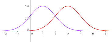
where the x axis represent feature X and y-axis represent the possibility density function value.
We can see that two distributions have the overlapping region.

If we want to determine when to reject H0, we need a threshold of feature x (a vertical line) to separate H0 and H1.
Then to find such threshold, it involves the concept of significant level and p-value

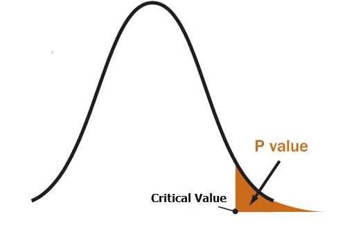
P-value

What is p-value

P-value is the probability under the assumption of no effect or no difference (null hypothesis H0), of obtaining a result equal to or more extreme than what was actually observed. (在H0=true的假设前提下/H0=True的distribution下,取得比目前的evidence/observation 同等极端或更加极端更加极端的事件的概率). The P stands for probability and measures how likely it is that any observed difference between groups is due to chance.

In other words, P-value actually measure how strong the evidence is to reject H0. If P-value is larger, then the strenght of evidence to reject H0 is weaker. Otherwise, the strenght is stronger.

Example: Assume I am sampling a random number from a range [-1000, 1000] and assumes that the distributions of number in this range is normal distribution with mean =0. An observation is a sample with value =900. Then the P-value of this observation is the possibility of obtaining sample >=900. In the plot of possbility density function, P-value represents the area under curve in X>=900.

Significant level and confidence level

In order to determine whether reject H0 or not, we need to define a threshold for P-value and this leads to the concepts of significant level and confidence level.

Significant level

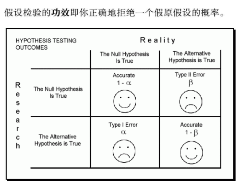
“Significant” means how significant the difference between groups is so that we should consider such difference is meaningful. Significant level is usually notated as $\alpha$ and $\alpha$=P(reject H0 | H0 =true). significant level is the possibility of rejecting H0 when H0 is true.

Moreover, the error that rejecting H0 when H0 is true is called Type I error. Hence Significant level is also the possibility of the occurence of Type I error / Type I error rate (Significant error = Type I error)

confidence level

Confidence level is the possibility of retaining H0 when H0 is true. Hence we know that confidence level = 1- significant level = $1-\alpha$
Confidence interval is the region outside the shadow region of $\alpha$ in the distribution of H0=true.

In the possibility density function, We can see that the shadow region in the figure represent a single side significant level (as it is possibility, in density function, it represents an area). Then the area of shadow region = $\alpha$

When to reject H0

if P-value < $\alpha$, we reject H0 and choose H1. if P-value >=$\alpha$, retain H0

if an observation X on the x-axis is outside of shadow region, that is, P-value, P(x>=X) is greater than or equal to significant level, then we think observation X is common under null hypothesis H0 and we can not use X to reject H0.

if P-value is smaller than significant level / observation X fall inside shadow region, then the difference between groups will be considered and we reject H0 and choose H1. In other words, the observation X is too rare so that we don’t consider it satisfies null hypothesis and hence it becomes a contradiction to reject H0.

Note:

significant level and confidence level is set by user and the value of significant level is usually 0.05 or 5%. This also means that users assume the possibility of rejecting a true hypothesis H0 due to some extreme cases under current observation method should be smaller than significant level $\alpha$.

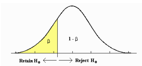
Retain region and power

Now, we are considering the alternative hypothesis H1 rather than H0. Assume the distribution from H1 is normal distribution as well.

Beta/retain region

The yellow region of distribution of H1=True is the retain region for H0 and the area of the yellow region is $\beta$, which represents the possibility of retaining H0 when H1=True. If the observation value X on x-axis falls into the yellow region, then we retain Hypothesis H0.
$\beta$ = P(retain H0 | H0 = False) = Type II error rate ( possibility to retain H0 when H0 is false under assumption H1=True)

Power

power is possibility of rejecting null hypothesis H0 and power = 1- $\beta$.
if power is set to be larger, then testing could be easier to detect and reject false Null hypothesis. But if power is too large, it would reject a good hypothesis as well, despite the null hypothesis is true.

Note that there is a tradeoff between $\alpha$ and $\beta$. When we set smaller $\alpha$ value to decrease the Type I error rate (reject H0 when H0 is True), then $\beta$ / Type II Error rate (retain H0 when H0 is False)will increase . Usually $\beta$ is not set by user, but it can be calculated using p-value and $\alpha$. Usually $\beta$ is around 20%

Type I and Type II Error

Now Let’s consider the distributions of hypothesis that H0=True (left) and the hypothesis that H1 = True (right) Together. Both distributions are estimated by sampling.

Since the yellow region $\beta$ in distribution of H1= True and confidence region of distribution of H0 = True represent the regions to retain H0, we can put two distribution together. Then the vertical line separates the region of retaining H0 (left) and rejecting H0 (right).

Remember that $\alpha$ = Type I error rate = P(reject H0 | H0 = True) and $\beta$ = Type II error rate = P(retain H0 | H0 = False) and there is trade-off between Type I error rate and Type II error rate.

When we lower significant level $\alpha$, $\beta$ will increase. In other words, lowering threshold to reject H0 can increase possibility of retaining H0, but also null hypothesis H0 may not be true, in this case, rate of accepting False H0 will increase.

Factors affecting Power and $\beta$

Size of the effect / effect size

The size of the effect is the distance between the mean of null hypothesis distributions and the mean of true distribution.
If $\alpha$ is fixed, then Greater the size of effect is, smaller $\beta$ / Type II error rate is and more different two distributions are.

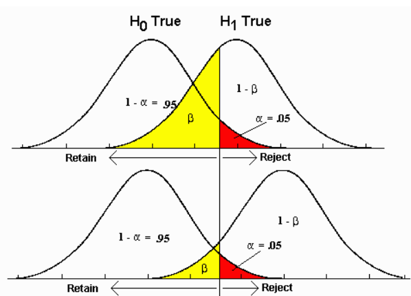
We can see that the first figure has the effect size smaller than the effect size in second figure, as the $\beta$ in the top figure is larger than the bottom one.

Assume distribution of H0=True is estimated from samples and the real distribution of population is distribution of H1=True. Then Equation to compute size of effect is: effect size = $\frac{\mu_{H0} -\mu_{H1} }{\sigma_{H1}}$
where $\mu_{H0}$, $\mu_{H1}$ are mean of H0, H1 $\sigma_{H1}$ is standard variance of distribution of H1=True.

Note that effect size can be computed, but can not be controlled by users directly. It depends on the samples and population.

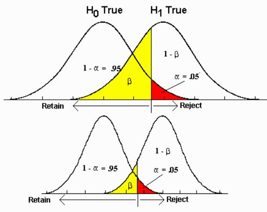
Size of samples
The sample size controls the variance of a distribution (width of distribution) and hence can affect $\beta$ / Type II error rate. In the following figure, when $\alpha$ and means of two distributions H0=True, H1 = True are fixed, large sample size is, smaller variance is and smaller $beta$ / Type II error is

Control Type I error $\alpha$

To control Type I error rate/ $\alpha$, we can change $\alpha$ directly. Decrease $\alpha$ is to decrease Type I error rate (rejecting H0 when H0 =True)
Usually $\alpha$ is set to be 0.05 or 0.01

Control Type II error $\beta$ or (1- power)

Since there is trade-off between Type I error rate $\alpha$ and Type II error rate $\beta$, we can increase $\alpha$ to decrease $\beta$ and increase power
Increase sample size to decrease variance of distribution to decrease $\beta$, the rate of accepting H0 when H0=False.

Two-tailed Hypthesis Testing

The hypothesis testing above is called single-tailed hypothesis testing, since we only consider the significant level $\alpha$ in on one side only. In the figure below $H_a: \mu <\mu_0 $ means the sample mean $\mu$ is smaller than population mean $\mu_0$. In single-tailed test, we only consider one-side of relationship and disregard another side

Now we consider the Two-tailed Hypothesis testing with the sum of area of left tail and right tail in distribution of H0 equal to $\alpha$. The figure is shown below. In two-tailed test, we regard the extreme cases on both sides.

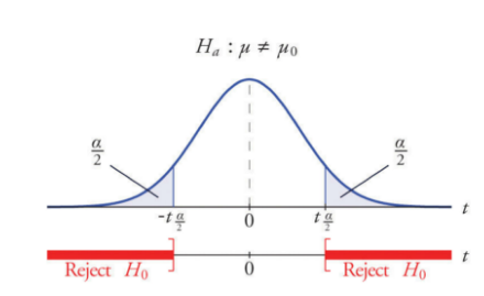
*We reject H0 when 2P-value< $\alpha$ or P-value < $\frac{\alpha}{2}$ in Two-tailed Hypothesis Testing**

For example, we want to analysis how tall the people are in a region. Then

Example 1:
H0: the mean tall of population = 1.75 m
H1: the mean tall of population is not equal to 1.75 m.
Observation: the mean of a sample group of people = 1.9m.
In this case, if we care whether tall mean of people is >1.75m or <=1.75m, then we use two-tailed test and compare P-value with $\frac{\alpha}{2}$

Example 2:
H0: the mean tall of population = 1.75 m
H1: the mean tall of population is greater than 1.75 m.
Observation: the mean of a sample group of people = 1.9m.
If we care if tall mean of people >1.75m or not only, then we use one-tailed test and compare P-value with $\alpha$.

Example 3:
H0: the mean tall of population = 1.75 m
H1: the mean tall of population is less than or equal to 1.75 m.
Observation: the mean of a sample group of people = 1.5m.
In this case, we care if mean <=1.75m or not only, then we use one-tailed test again.

Choosing which tail in one-tailed test depends on the observation and your alternative hypothesis H1.

When to use single-tailed test or two-tailed test

Choosing two-tailed test when:
- when you care extreme cases on both sides of distribution without direction
- when effects exist on both sides based on your observations.
- Note that if effect exists on two sides, but we choose single-tailed test, then the expected significant level =$\alpha$ but we choose $\frac{\alpha}{2}$, this may increase Type II error rate and decrease power as we decrease $\alpha$
Choosing one-tailed test when:
- when you care one side of effect / extreme cases on one side only
- when effects exist on only one side based on your observations
- Note that if effect exists on two tails and we choose one-tailed test, then expected significant level =$\frac{\alpha}{2}$, but we use $\alpha$ instead, this may increase Type I error rate.

Methods to compute p-value

The common methods to compute P-value as follow, I will introduce them in the next article

z-test
- Z-distribution/normal distribution
- Assume data follow normal distribution
- usually used with continuous variables
t-test
- Use t-distribution
- usually used with continuous variables
Pearson’s Chi-Square score
- Use Chi sqare distribution (Square Sum of multiple normal distribution)
- Used to measure independence between two variables
- Can be used for continuous variables or discrete variables

Factors affecting Hypothesis testing

Sample size
As mentioned before, sample size can affect $\beta$, type II error rate (retain H0/ can not reject H0 when H0 is false).
Randomized Experiment
In order to obtain representative samples from population in hypothesis testing to compute the p-value, we need to avoid sampling in bias. This leads to randomized experiment. There are some important terms in randomized experiment:
- Random sampling
  Random sampling is to obtain get some representative samples from the population (full traffic) randomly. If the samples are not obtained randomly, it could be biased which can affect the distribution of sample data even sample size is large
- Randomization / Random assignment
  Randomization is how you allocate samples to groups in experiment. It alleviates the bias that might cause a systematic difference between groups unrelated to the treatment itself.
  
  For example, If I want to test if the new UI design of a software can get higher ClickThrough rate (CRT) from users. Then I compare a group of users who use the new UI, called treatment group with another group of users who use original UI, called controlled group. Then After I randomly sample the users from different region, the way that I randomly assign those users to treatment group or controlled group is randomization/ random assignment.
- Confounding factor /variable
  Confounding factor is the factor that correlates with the independent and dependent variable confuse the effects and impact the results of experiments.
  Randomization of experiments is the key to controlling for confounding variables in machine learning experiments.

Summary to use Hypothesis testing

Specify a Null Hypothesis H0 and alternative Hypothesis H1 based on some observations (H0 and H1 should be mutually exclusive). Choose one-tailed test or two-tailed test based on H0 and H1
Specify significant level $\alpha$
Compute P-value based on dataset (t-test/t-statistic, z-test, F-statistic,Chi-square test)
Compare P-value with significant level $\alpha$. If P-value >= $\alpha$, retain H0 (NOT accept !). If P-value < $\alpha$, reject H0 and retain H1