2021-06-15Deep Learning28 minutes read (About 4125 words) 0 visits

GNN-1-Basic

1. Graph Basic

参考资料: “Chapter 2 - Foundations of Graphs, Deep Learning on Graphs”

图的表示

定义一（图）：

一个图被记为 $\mathcal{G}={\mathcal{V}, \mathcal{E}}$，其中 $\mathcal{V}={v_{1}, \ldots, v_{N}}$ 是数量为 $N=|\mathcal{V}|$ 的结点的集合， $\mathcal{E}={e_{1}, \ldots, e_{M}}$ 是数量为 $M$ 的边的集合。
图用节点表示实体（entities ），用边表示实体间的关系（relations）。
节点和边的信息可以是类别型的（categorical），类别型数据的取值只能是哪一类别。一般称类别型的信息为标签（label）。
节点和边的信息可以是数值型的（numeric），类别型数据的取值范围为实数。一般称类别型的信息为属性（attribute）。
大部分情况中，节点含有信息，边可能含有信息。

定义二（图的邻接矩阵）：

给定一个图$\mathcal{G}={\mathcal{V}, \mathcal{E}}$，其对应的邻接矩阵被记为$\mathbf{A} \in{0,1}^{N \times N}$。$\mathbf{A}_{i, j}=1$表示存在从结点$v_i$到$v_j$的边，反之表示不存在从结点$v_i$到$v_j$的边。
在无向图中，从结点$v_i$到$v_j$的边存在，意味着从结点$v_j$到$v_i$的边也存在。因而无向图的邻接矩阵是对称的。
在无权图中，各条边的权重被认为是等价的，即认为**各条边的权重为$1$**。
对于有权图，其对应的邻接矩阵通常被记为$\mathbf{W} \in{0,1}^{N \times N}$，其中$\mathbf{W}{i, j}=w{ij}$表示从结点$v_i$到$v_j$的边的权重。若边不存在时，边的权重为$0$。

一个无向无权图的例子：

其邻接矩阵(Adjacency matrix)为：

$$
\mathbf{A}=(\begin{array}{lllll}
0 & 1 & 0 & 1 & 1 \\
1 & 0 & 1 & 0 & 0 \\
0 & 1 & 0 & 0 & 1 \\
1 & 0 & 0 & 0 & 1 \\
1 & 0 & 1 & 1 & 0
\end{array})
$$

二、图的属性

定义三（结点的度，degree）：

对于有向有权图，结点$v_i$的出度（out degree）等于从$v_i$出发的边的权重之和，结点$v_i$的入度（in degree）等于从连向$v_i$的边的权重之和。
无向图是有向图的特殊情况，结点的出度与入度相等。
无权图是有权图的特殊情况，各边的权重为$1$，那么结点$v_i$的出度（out degree）等于从$v_i$出发的边的数量，结点$v_i$的入度（in degree）等于从连向$v_i$的边的数量。
结点$v_i$的度记为$d(v_i)$，入度记为$d_{in}(v_i)$，出度记为$d_{out}(v_i)$。

定义四（邻接结点，neighbors）：

结点$v_i$的邻接结点为与结点$v_i$直接相连的结点，其被记为**$\mathcal{N(v_i)}$**。
结点$v_i$的$k$跳远的邻接节点（neighbors with $k$-hop）指的是到结点$v_i$要走$k$步的节点（一个节点的$2$跳远的邻接节点包含了自身）。

定义五（行走，walk）：

$walk(v_1, v_2) = (v_1, e_6,e_5,e_4,e_1,v_2)$，这是一次“行走”，它是一次从节点$v_1$出发，依次经过边$e_6,e_5,e_4,e_1$，最终到达节点$v_2$的“行走”。
下图所示为$walk(v_1, v_2) = (v_1, e_6,e_5,e_4,e_1,v_2)$，其中红色数字标识了边的访问序号。
在“行走”中，节点是运行重复的。

定理六：

有一图，其邻接矩阵为 $\mathbf{A}$, $\mathbf{A}^{n}$为邻接矩阵的$n$次方，那么$\mathbf{A}^{n}[i,j]$等于从结点$v_i$到结点$v_j$的长度为$n$的行走的个数。

定义七（路径，path）：

“路径”是结点不可重复的“行走”。

定义八（子图，subgraph）：

有一图$\mathcal{G}={\mathcal{V}, \mathcal{E}}$，另有一图$\mathcal{G}^{\prime}={\mathcal{V}^{\prime}, \mathcal{E}^{\prime}}$，其中$\mathcal{V}^{\prime} \in \mathcal{V}$，$\mathcal{E}^{\prime} \in \mathcal{E}$并且$\mathcal{V}^{\prime}$不包含$\mathcal{E}^{\prime}$中未出现过的结点，那么$\mathcal{G}^{\prime}$是$\mathcal{G}$的子图。

定义九（连通分量，connected component）：

给定图$\mathcal{G}^{\prime}={\mathcal{V}^{\prime}, \mathcal{E}^{\prime}}$是图$\mathcal{G}={\mathcal{V}, \mathcal{E}}$的子图。记属于图$\mathcal{G}$但不属于$\mathcal{G}^{\prime}$图的结点集合记为$\mathcal{V}/\mathcal{V}^{\prime}$ 。如果属于$\mathcal{V}^{\prime}$的任意结点对之间存在至少一条路径，但不存在一条边连接属于$\mathcal{V}^{\prime}$的结点与属于$\mathcal{V}/\mathcal{V}^{\prime}$的结点，那么图$\mathcal{G}^{\prime}$是图$\mathcal{G}$的连通分量。

定义十（连通图，connected graph）：

当一个图只包含一个连通分量，即其自身，那么该图是一个连通图。

定义十一（最短路径，shortest path）：

$v_{s}, v_{t} \in \mathcal{V}$ 是图$\mathcal{G}={\mathcal{V}, \mathcal{E}}$上的一对结点，结点对 $v_{s}, v_{t} \in \mathcal{V}$ 之间所有路径的集合记为 $P_{\mathrm{st}}$ 。结点对$v_{s}, v_{t}$之间的最短路径 $p_{\mathrm{s} t}^{\mathrm{sp}}$为$\mathcal{P}_{\mathrm{st}}$ 中长度最短的一条路径，其形式化定义为$$
p_{\mathrm{s} t}^{\mathrm{sp}}=\arg \min {p \in \mathcal{P}{\mathrm{st}}}|p|
$$其中，$p$表示$\mathcal{P}_{\mathrm{st}}$中的一条路径，$|p|$是路径$p$的长度。

定义十二（直径，diameter）：

给定一个连通图$\mathcal{G}={\mathcal{V}, \mathcal{E}}$，其直径为其所有结点对之间的最短路径的最小值，形式化定义为

$$
diameter(\mathcal{G})=\max_{v_{s}, v_{t} \in \mathcal{V}} \min_{p \in \mathcal{P}_{s t}}|p|
$$

定义十三（拉普拉斯矩阵，Laplacian Matrix）：

给定一个图$\mathcal{G}={\mathcal{V}, \mathcal{E}}$，其邻接矩阵为$A$，其拉普拉斯矩阵定义为$\mathbf{L=D-A}$，其中$\mathbf{D=diag(d(v_1), \cdots, d(v_N))}$。

定义十四（对称归一化的拉普拉斯矩阵，Symmetric normalized Laplacian）：

给定一个图$\mathcal{G}={\mathcal{V}, \mathcal{E}}$，其邻接矩阵为$A$，其规范化的拉普拉斯矩阵定义为

$$
\mathbf{L=D^{-\frac{1}{2}}(D-A)D^{-\frac{1}{2}}=I-D^{-\frac{1}{2}}AD^{-\frac{1}{2}}}
$$

三、图的种类

同质图（Homogeneous Graph）：只有一种类型的节点和一种类型的边的图。
异质图（Heterogeneous Graph）：存在多种类型的节点和多种类型的边的图。
二部图（Bipartite Graphs）：节点分为两类，只有不同类的节点之间存在边。

四、图结构数据上的机器学习

节点预测：预测节点的类别或某类属性的取值
1. 例子：对是否是潜在客户分类、对游戏玩家的消费能力做预测
边预测：预测两个节点间是否存在链接
1. 例子：Knowledge graph completion、好友推荐、商品推荐
图的预测：对不同的图进行分类或预测图的属性
1. 例子：分子属性预测
节点聚类：检测节点是否形成一个社区
1. 例子：社交圈检测
其他任务
1. 图生成：例如药物发现
2. 图演变：例如物理模拟
3. ……

五、应用神经网络于图面临的挑战

在学习了简单的图论知识，我们再来回顾应用神经网络于图面临的挑战。

过去的深度学习应用中，我们主要接触的数据形式主要是这四种：矩阵、张量、序列（sequence）和时间序列（time series），它们都是规则的结构化的数据。然而图数据是非规则的非结构化的，它具有以下的特点：

任意的大小和复杂的拓扑结构；
没有固定的结点排序或参考点；
通常是动态的，并具有多模态的特征；
图的信息并非只蕴含在节点信息和边的信息中，图的信息还包括了图的拓扑结构。

以往的深度学习技术是为规则且结构化的数据设计的，无法直接用于图数据。应用于图数据的神经网络，要求

适用于不同度的节点；
节点表征的计算与邻接节点的排序无关；
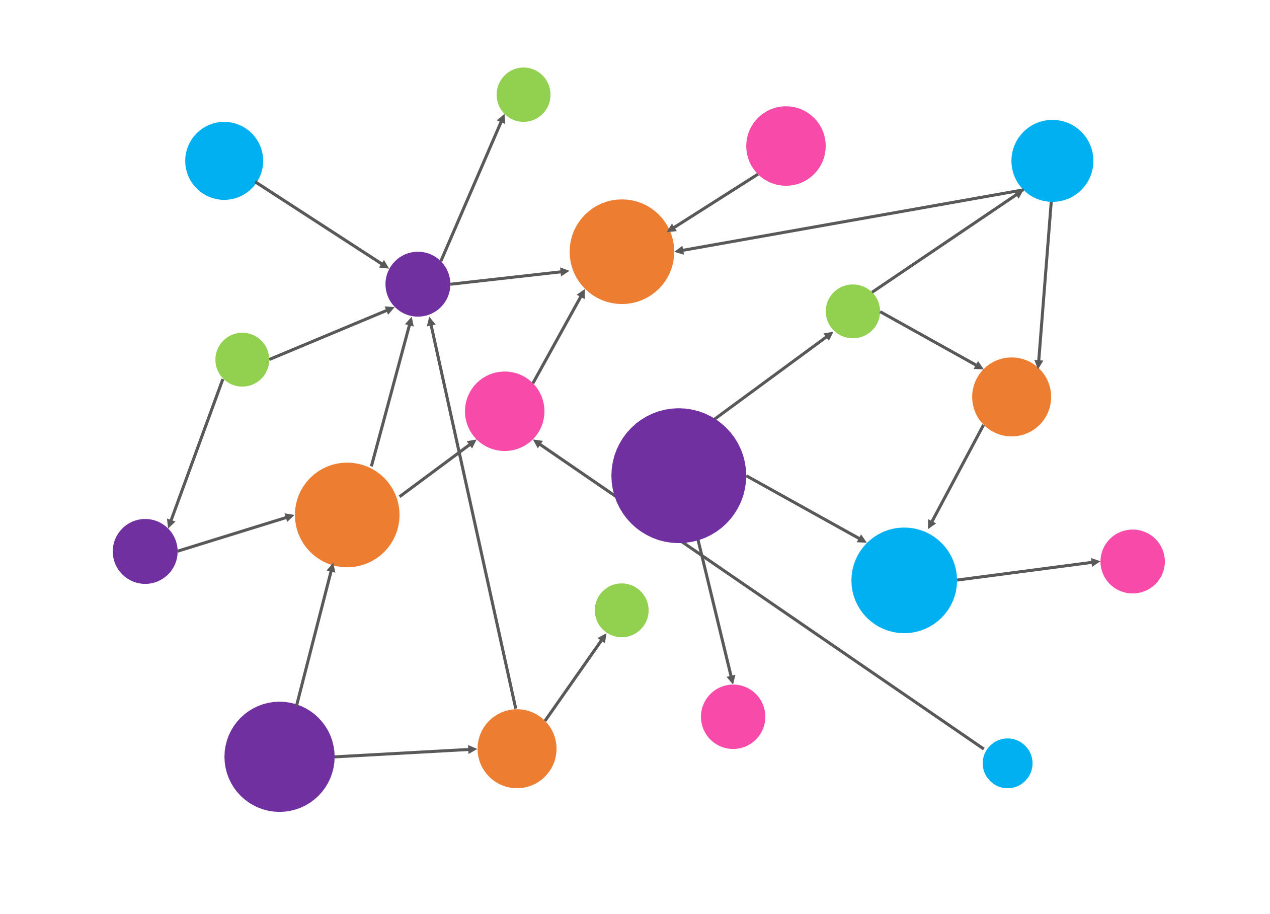
不但能够根据节点信息、邻接节点的信息和边的信息计算节点表征，还能根据图拓扑结构计算节点表征。下面的图片展示了一个需要根据图拓扑结构计算节点表征的例子。图片中展示了两个图，它们同样有俩黄、俩蓝、俩绿，共6个节点，因此它们的节点信息相同；假设边两端节点的信息为边的信息，那么这两个图有一样的边，即它们的边信息相同。但这两个图是不一样的图，它们的拓扑结构不一样。

六、结语

在此篇文章中，我们学习了简单的图论知识。对于学习此次组队学习后续的内容，掌握这些图论知识已经足够。如果有小伙伴希望掌握更多的图论知识可以参阅参考文献“Chapter 2 - Foundations of Graphs, Deep Learning on Graphs”。

参考资料

Chapter 2 - Foundations of Graphs, Deep Learning on Graphs

2. Practice

先看看torch的version 以及torch使用的cuda version

1 2	import torch torch.version.cuda, torch.__version__

('11.1', '1.8.1')

根据它们的版本对下面的html的名字调整，这里我用的是torch cuda 是 11.1，torch 是1.8.1所以用torch-1.8.1+cu111.html

# pip install torch-scatter -f https://pytorch-geometric.com/whl/torch-1.8.1+cu111.html --no-cache
# pip install torch-sparse -f https://pytorch-geometric.com/whl/torch-1.8.1+cu111.html --no-cache
# pip install torch-cluster -f https://pytorch-geometric.com/whl/torch-1.8.1+cu111.html --no-cache
# pip install torch-spline-conv -f https://pytorch-geometric.com/whl/torch-1.8.1+cu111.html --no-cache
# pip install torch-geometric

测试安装好的torch_geometric,另外也下载cora数据进行测试

from torch_geometric.datasets import KarateClub

dataset = KarateClub()
data = dataset[0]  # Get the first graph object.
print(data)
print('==============================================================')
print(f'Number of node features:{data.num_node_features}') # 节点属性的维度
print(f'Number of node features: {data.num_features}')
# 同样是节点属性的维度
print(f'Number of edge features: {data.num_edge_features}') # 边属性的维度
print(f'Average node degree: {data.num_edges /data.num_nodes:.2f}') # 平均节点度
print(f'if edge indices are ordered and do not contain duplicate entries.: {data.is_coalesced()}') # 是否边是有序的同时不含有重复的边
print(f'Number of training nodes: {data.train_mask.sum()}') # 用作训练集的节点
print(f'Training node label rate: {int(data.train_mask.sum()) / data.num_nodes:.2f}') #用作训练集的节点的数量
print(f'Contains isolated nodes: {data.contains_isolated_nodes()}') # 此图是否包含孤立的节点
print(f'Contains self-loops: {data.contains_self_loops()}') # 此图是否包含自环的边
print(f'Is undirected: {data.is_undirected()}') # 此图 是否是无向图

Data(edge_index=[2, 156], train_mask=[34], x=[34, 34], y=[34])
==============================================================
Number of node features:34
Number of node features: 34
Number of edge features: 0
Average node degree: 4.59
if edge indices are ordered and do not contain duplicate entries.: True
Number of training nodes: 4
Training node label rate: 0.12
Contains isolated nodes: False
Contains self-loops: False
Is undirected: True

1	! wget https://github.com/kimiyoung/planetoid/raw/master/data/ind.cora.x

--2021-06-14 13:56:45--  https://github.com/kimiyoung/planetoid/raw/master/data/ind.cora.x
Resolving github.com (github.com)... 140.82.112.4
Connecting to github.com (github.com)|140.82.112.4|:443... connected.
HTTP request sent, awaiting response... 302 Found
Location: https://raw.githubusercontent.com/kimiyoung/planetoid/master/data/ind.cora.x [following]
--2021-06-14 13:56:46--  https://raw.githubusercontent.com/kimiyoung/planetoid/master/data/ind.cora.x
Resolving raw.githubusercontent.com (raw.githubusercontent.com)... 185.199.110.133, 185.199.111.133, 185.199.108.133, ...
Connecting to raw.githubusercontent.com (raw.githubusercontent.com)|185.199.110.133|:443... connected.
HTTP request sent, awaiting response... 200 OK
Length: 22119 (22K) [application/octet-stream]
Saving to: ‘ind.cora.x’

ind.cora.x          100%[===================>]  21.60K  --.-KB/s    in 0s      

2021-06-14 13:56:46 (69.8 MB/s) - ‘ind.cora.x’ saved [22119/22119]

from torch_geometric.datasets import Planetoid
dataset = Planetoid(root='./dataset/Cora', name='Cora')
# Cora()
len(dataset)
# 1
dataset.num_classes
# 7
dataset.num_node_features
# 1433

Downloading https://github.com/kimiyoung/planetoid/raw/master/data/ind.cora.x
Downloading https://github.com/kimiyoung/planetoid/raw/master/data/ind.cora.tx
Downloading https://github.com/kimiyoung/planetoid/raw/master/data/ind.cora.allx
Downloading https://github.com/kimiyoung/planetoid/raw/master/data/ind.cora.y
Downloading https://github.com/kimiyoung/planetoid/raw/master/data/ind.cora.ty
Downloading https://github.com/kimiyoung/planetoid/raw/master/data/ind.cora.ally
Downloading https://github.com/kimiyoung/planetoid/raw/master/data/ind.cora.graph
Downloading https://github.com/kimiyoung/planetoid/raw/master/data/ind.cora.test.index
Processing...
Done!





1433

data = dataset[0]
# Data(edge_index=[2, 10556], test_mask=[2708],
# train_mask=[2708], val_mask=[2708], x=[2708,1433], y=[2708])
data.is_undirected()
# True
data.train_mask.sum().item()
# 140
data.val_mask.sum().item()
# 500
data.test_mask.sum().item()

3. Torch_geometric Data set 使用

在 from torch_geometric.data import Data调用 Data class之后， Data创建的实例时的输入有以下:

data.x:节点的数据矩阵，这个矩阵的大小为 [num_nodes, num_node_features]
data.edge_index: 图的连接信息，存放在Coordinate format (COO format) 它的矩阵大小为[2, num_edges] data type是torch.long
data.edge_attr: 边的特征矩阵它的shape是 [num_edges, num_edge_features]
data.y: 用于训练图神经网络的target，它能够有不同的形状，可以是对应节点特征的target，也可以是对应整个图的target, e.g., node-level targets of shape [num_nodes, *] or graph-level targets of shape [1, *]
data.pos: 节点的位置信息，它的shape是 [num_nodes, num_dimensions]，每一行代表有一个node的位置

详情可以参考官方文档: https://pytorch-geometric.readthedocs.io/en/latest/notes/introduction.html

4. Assignment

这里实践一遍，通过把Data class继承自定义自己的graph dataset，这个和torch的自定义dataset的创建很相似。

题目: 请通过继承Data 类实现一个类，专门用于表示“机构-作者-论文”的网
络。该网络包含“机构“、”作者“和”论文”三类节点，以及“作者-机构“和
“作者-论文“两类边。对要实现的类的要求：1）用不同的属性存储不同
节点的属性；2）用不同的属性存储不同的边（边没有属性）；3）逐一
实现获取不同节点数量的方法。

from torch_geometric.data import Data

import numpy as np

class MyGraphData(Data):
    def __init__(self, data, labels, **args ):
        """
        data: structural data, a table. Each column of table is one type of node
            so in this case: we have author, department, paper 3 different types of node.
            each value in the table represent a data value/ID value in a data node in graph
            Example:  
            author  depart  paper
              1       1       1
              2       1       2
              Then author #1 in department 1 writes 1 paper
              author #2 in department 2 writes 2 papers
              This is a heterogenuous graph
              
            I consider the missing value and isolated nodes in the input data as well.
        **args: other args passed to the Graph Data
        
        """
        super(MyGraphData, self).__init__()
        self.data = data
        self.edge_index = None
        self.x = None
        self.y = None
        self.node_list = []
        self.labels = labels
        self.create_graph(self.data)
        pass
    def create_graph(self,data):
        self.edge_index = []
        for row in self.data.values:
            # we get 3 nodes here, each has type / target: department, author, paper respectively
            dept = row[0]
            author = row[1]
            paper = row[2]
            print(dept, author, paper)
            dept_node_index = self.__add_node(self.node_list, dept, self.labels['dept']) #if dept !=None else None
            author_node_index = self.__add_node(self.node_list, author, self.labels['author']) #if author !=None else None
            paper_node_index = self.__add_node(self.node_list, paper, self.labels['paper']) #if paper !=None else None
            
            # add undirected author-department edge
            if dept_node_index!=None and author_node_index!=None:
                self.edge_index.append([dept_node_index, author_node_index])
                self.edge_index.append([ author_node_index,dept_node_index])
            
            # add undirected author-paper edge
            if author_node_index!=None and paper_node_index!=None:
                self.edge_index.append([ author_node_index,paper_node_index])
                self.edge_index.append([ paper_node_index,author_node_index])
                
        # first row = from node ,  second row = to node
        self.edge_index = torch.tensor(np.array(self.edge_index).T, dtype= torch.long)
        
        # gather value of each node into a feature matrix x
        self.x = torch.tensor([node[0] for node in self.node_list], dtype= torch.float)
        
        # gather target for each node
        self.y = torch.tensor([node[1] for node in self.node_list], dtype = torch.float)
        return self.x,  self.edge_index, self.y
            
            
            
    def __add_node(self, node_ls, node, target):
        if node == None or np.isnan(node):
            return None
        if node_ls.count([node, target]) ==0:
            # check if node exists
            node_ls.append([node, target])
        # return the index of the unique node
        node_idx = node_ls.index([node, target])
        return node_idx
    @property
    def dept_nums(self):
        return self.data['dept'].nunique()

    @property
    def author_nums(self):
        return self.data['author'].nunique()

    @property
    def paper_nums(self):
        return self.data['paper'].nunique()
    @property
    def isolated_nodes(self):
        iso_nodes = []
        for n in range(len(self.node_list)):
            if n not in self.edge_index:
                iso_nodes.append(self.node_list[n])
        return iso_nodes

# Data(edge_index=[2, 4], x=[3, 1])
import pandas as pd
x = pd.DataFrame(data= [[1,1,1],[2,2,1],[None, None, 3]], columns=["dept","author","paper"])
data = MyGraphData(data = x, labels = {"dept":0,"author":1,"paper":2})

1.0 1.0 1.0
2.0 2.0 1.0
nan nan 3.0

print("Test Results:")
print(f"Number of authors: {data.author_nums}")
print(f"Number of papers: {data.paper_nums}")
print(f"Number of departments: {data.dept_nums}")
print(f"Number of isolated nodes: {len(data.isolated_nodes)}")
print(f"Edge index: {data.edge_index}")
print(f"x representation matrix: {data.x}")
print(f"Node index [value, label]: {data.node_list}")

Test Results:
Number of authors: 2
Number of papers: 2
Number of departments: 2
Number of isolated nodes: 1
Edge index: tensor([[0, 1, 1, 2, 3, 4, 4, 2],
        [1, 0, 2, 1, 4, 3, 2, 4]])
x representation matrix: tensor([1., 1., 1., 2., 2., 3.])
Node index [value, label]: [[1.0, 0], [1.0, 1], [1.0, 2], [2.0, 0], [2.0, 1], [3.0, 2]]

1
2

#GNN Graph

GNN-1-Basic

1. Graph Basic

图的表示

二、图的属性

三、图的种类

四、图结构数据上的机器学习

五、应用神经网络于图面临的挑战

六、结语

参考资料

2. Practice

3. Torch_geometric Data set 使用

4. Assignment

Comments

Links

Categories

Tags

Recent

Archives

Subscribe to Updates

Catalogue