GNN-3-NodeEmbedding
Node Embedding and Node Prediction
1. Introduction
首先回顾一下上一篇文章关于MessagePassing的GNN的内容。在GNN的MessagePassing里面,每个node代表一个subject,然后edge代表subject之间的关系。而MessagePassing一句话总结就是让每个node的特征(node representation 或node embedding)通过对应的neighbor nodes的信息进行聚集并用于更新每个node
的信息,从而学习到更好的node embedding表达。之后我们可以对学习到的node embedding里面每个node的特征向量输入到classifier里面进行node classification识别subject的类别。除了node classification外,node embedding还能用来做edge classification, graph classification 等任务。
而这次项目的目的是要实现GNN图神经网络并进行实践应用到Cora (scientific publications)科学文献dataset里面,并对每篇文章进行分类和预测文章的类别。这次的项目的大概流程是:
- Introduction to Cora Dataset: 简单介绍一下Cora论文数据集的构成
- Data Visualization: 对Cora数据集的node representation 和class 进行可视化
- Modeling and training: 搭建和训练MLP, GCN, GAT等模型对node 进行classification以及测试
- Visualize learned node representation: 将学到的node representation进行可视化分析每个类分布的不同
- Assignment: 尝试其他不同的Dataset看一下不同GNN的效果
- Conclusion: 总结一下学到什么
2. Data Description
这里先来介绍Coras Dataset的内容,Coras Dataset 的解释可以从官网找到: https://linqs.soe.ucsc.edu/data
Coras dataset content:
- Number of nodes: 2708 nodes. 每个node代表一篇论文
- Number of edges/links: 5429条无向的边,如果用有向的边表示就是10556条
- Number of class: 8. 总共有7个类别的论文
- Dimension of node representation: 1433. 字典的大小为1433每个词用0,1 表示文章有没有那个词. 每篇文章的node representation就有1433
1 | from torch_geometric.datasets import Planetoid |
Dataset: Cora():
======================
Number of graphs: 1
Number of features: 1433
Number of classes: 7

Data(edge_index=[2, 10556], test_mask=[2708], train_mask=[2708], val_mask=[2708], x=[2708, 1433], y=[2708])
======================
Number of nodes: 2708
Number of edges: 10556
Average node degree: 3.90
Number of training nodes: 140
Training node label rate: 0.05
Contains isolated nodes: False
Contains self-loops: False
Is undirected: True
1 | data.train_mask,data.y.unique() |
(tensor([ True,  True,  True,  ..., False, False, False]),
 tensor([0, 1, 2, 3, 4, 5, 6]))
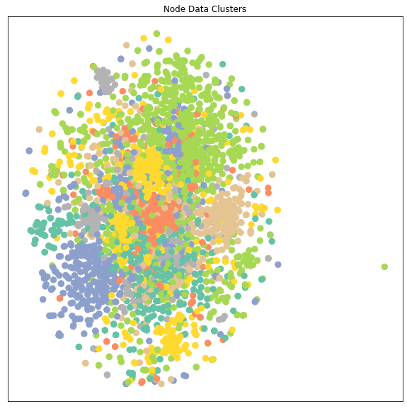
2. Data Visualization
这里简单用TSNE的降维算法把1433 维的node representation降到2维从而来显示每个class的数据的分布, 每种颜色代表一个class。从下面每种颜色的点的分布来看,在学习之前的不同类别的node representation是很难区分开来的,所以很多节点的特征都混在一起
1 | import matplotlib.pyplot as plt |
1 | data.x.shape, data.y.shape |
(torch.Size([2708, 1433]), torch.Size([2708]))
1 | visualize(data.x,data.y,"Node Data Clusters") |
3. 用不同GNN对node embedding进行学习
这里先简单来设计training, testing 的通用函数, 之后尝试用以下不同的模型进行学习和对比:
- MLP
- GNN
- GAT
- GraphSAGE
1 | def train(model, criterion, optimizer,data, use_mask=True): |
3.1 MLP
1 | import torch |
Model Strucutre:
MLP(
  (lin1): Linear(in_features=1433, out_features=16, bias=True)
  (lin2): Linear(in_features=16, out_features=7, bias=True)
)
Epoch: 020, Loss: 1.7441
Epoch: 040, Loss: 1.2543
Epoch: 060, Loss: 0.8578
Epoch: 080, Loss: 0.6368
Epoch: 100, Loss: 0.5350
Epoch: 120, Loss: 0.4745
Epoch: 140, Loss: 0.4031
Epoch: 160, Loss: 0.3782
Epoch: 180, Loss: 0.4203
Epoch: 200, Loss: 0.3810

Test Accuracy: 0.5900
1 |
3.2 GCN
GCN Layer 公式如下:
$$
\mathbf{x}_ i^{(k)} = \sum_{j \in \mathcal{N}(i) \cup { i }} \frac{1}{\sqrt{\deg(i)} \cdot \sqrt{\deg(j)}} \cdot ( \mathbf{\Theta} \cdot \mathbf{x}_ j^{(k-1)} ),
$$
这里一些函数定义如下:
- $\phi(..)$: message函数GCN一样都是linear projection之后用degree进行normalization
- $\square(..)$ : aggregate 函数用 add
- $\gamma(..)$: update 函数是直接将aggregate后的结果输出
这里把MLP里面的linear layer换成是GCN layer
1 | import torch |
Model Architecture:
GCN(
  (conv1): GCNConv(1433, 16)
  (conv2): GCNConv(16, 7)
)
Epoch: 020, Loss: 1.7184
Epoch: 040, Loss: 1.3363
Epoch: 060, Loss: 1.0066
Epoch: 080, Loss: 0.7248
Epoch: 100, Loss: 0.5833
Epoch: 120, Loss: 0.5064
Epoch: 140, Loss: 0.4131
Epoch: 160, Loss: 0.3799
Epoch: 180, Loss: 0.3186
Epoch: 200, Loss: 0.3006

Test Accuracy: 0.8140
1 |
3.3 GAT (Graph Attention Network)
- paper link: https://arxiv.org/pdf/1710.10903.pdf
- Graph Attention Network 的attention公式如下:
$$
\alpha_ {i,j} = \frac{ \exp(\mathrm{LeakyReLU}(\mathbf{a}^{\top}
[\mathbf{W}\mathbf{h}_ i , \Vert , \mathbf{W}\mathbf{h}_ j]
))}{\sum_ {k \in \mathcal{N}(i) \cup { i }}
\exp(\mathrm{LeakyReLU}(\mathbf{a}^{\top}
[\mathbf{W} \mathbf{h}_ i , \Vert , \mathbf{W}\mathbf{h}_ k]
))}.
$$
节点信息更新
$$
\mathbf{h}_ i^{‘} = \sigma(\frac{1}{K} \sum_ {k=1}^K\sum_ {j \in N(i)} a_{ij}^{k}\mathbf{W}^k\mathbf{h}_ {i})
$$
实际上GAT就是在每个节点把邻居的信息聚合时根据邻居节点的node representation和这个节点的node representation的相似度对聚合的信息有侧重地聚合
其中每个参数的代表:
- $\mathbf{h}_i$: 节点 i的node representation。这个node representation可以是GNN的某一层的输出
- $\mathbf{W}$: shared linear transformation. 用于每个节点的共享的线性投映矩阵,所有节点都用相同的W进行投映
- $k \in \mathcal{N}(i) \cup { i }$: 第i个节点的邻居节点(包括第i个节点本身)。注意因为这里涉及两个sum,两个loop所以计算有点慢
- $\Vert$: 把两个向量拼接
1 | import torch |
Model Strucutre:
GAT(
  (conv1): GATConv(1433, 16, heads=1)
  (conv2): GATConv(16, 16, heads=1)
  (linear): Linear(in_features=16, out_features=7, bias=True)
)
Epoch: 020, Loss: 1.5780
Epoch: 040, Loss: 0.5588
Epoch: 060, Loss: 0.1466
Epoch: 080, Loss: 0.0755
Epoch: 100, Loss: 0.0585
Epoch: 120, Loss: 0.0351
Epoch: 140, Loss: 0.0406
Epoch: 160, Loss: 0.0292
Epoch: 180, Loss: 0.0285
Epoch: 200, Loss: 0.0287

Test Accuracy: 0.7230
对GAT做一点调参,提一下性能
- hidden_channels 用24时比小于16和大于32的时候好
- dropout=0.8时效果也更好,可能GAT里面的attention的机制容易对一部分特征overfitting
- epoch设置300更加长些也效果好点
- 这里调了下参数有了 6% 的提升
1 | model_gat = GAT(in_channel = dataset.num_features, classes = dataset.num_classes, hidden_channels = 24, dropout_r= 0.8) |
Model Strucutre:
GAT(
  (conv1): GATConv(1433, 24, heads=1)
  (conv2): GATConv(24, 24, heads=1)
  (linear): Linear(in_features=24, out_features=7, bias=True)
)
Epoch: 020, Loss: 1.6420
Epoch: 040, Loss: 0.7042
Epoch: 060, Loss: 0.4498
Epoch: 080, Loss: 0.2709
Epoch: 100, Loss: 0.2429
Epoch: 120, Loss: 0.1849
Epoch: 140, Loss: 0.2643
Epoch: 160, Loss: 0.1832
Epoch: 180, Loss: 0.2135
Epoch: 200, Loss: 0.1697
Epoch: 220, Loss: 0.1485
Epoch: 240, Loss: 0.1359
Epoch: 260, Loss: 0.1606
Epoch: 280, Loss: 0.1778
Epoch: 300, Loss: 0.1555

Test Accuracy: 0.7810
1 |
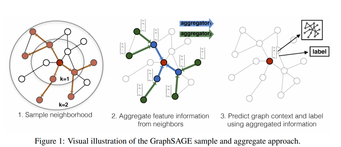
3.4. GraphSAGE (Sample and Aggregate Graph Embedding SAGE)
- Paper Link: https://arxiv.org/pdf/1706.02216.pdf
- 其他GNN的node embedding的学习方法都是假设了图里面所有node都是在训练时已经见到的并且有自己的特征数据作为训练集。 而在训练之后,当这些已经见过的node的特征值改变时,可以用GNN对它进行预测。但是实际问题里面,有可能有些node在训练时完全没有见过的(但是出现时会和其他已经见过的node存在link),因此不能在训练时用这些node的数据进行训练(这个有点像推荐系统的Embedding里面没有见过的userid或itemid的冷启动情况)。GraphSAGE就是用来解决这个问题
- GraphSAGE是一种 inductive的representation learning的方法,就是归纳法。它是用于预测之前没有见过的node的embed的ing的特征。它的主要思想是通过学习多个aggregate函数(paper里面提出来mean, LSTM, pooling 三个),然后这些aggregate函数用neighbor的信息来生成之前没有见过的node的embedding之后再做预测。下面是GraphSAGE的流程图:
GraphSAGE 的node embedding的其中一个生成公式为(还有其他用于生成embedding的aggregate函数公式可以参考原文):
$$
\mathbf{x}_ {i}^{‘} = \mathbf{W}_ {1}x_{i} + \textbf{mean}_ {j \in N(i)}(\mathbf{x}_{j})
$$GraphSAGE 的graph-based unsupervised loss function 定义为
$$
\mathbf{J}_ {G}(z_{u}) = -log(\sigma(\mathbf{z}_ {u}^{T}\mathbf{z}_ {v})) - \mathbf{Q} \cdot \mathbf{E}_ {v_ {n} \in P_ {n}(v)}log(\sigma(-\mathbf{z}_ {u}^{T} \mathbf{z}_ {v_{n}}))
$$
其中:
$j \in N(i)$ 为第i个节点的第j个neighbor节点
$v$ 是和 $u$ 在定长的random walk采样路径出现的节点
$Q$ 是负样本的个数, $P_{n}(v)$ 是负采样的分布
$z_{u}$是node representation特征
这里$\sigma()$里面计算的是节点和random walk采样时同时出现的其他节点的相似度。相似度越大,loss越小
GraphSAGE 的计算embedding算法流程如下:
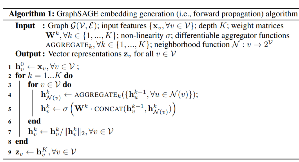
这里GraphSAGE的基本思路就是
- 先设定好K (iteration的次数又或者叫search depth搜索的深度)以及初始化没有见过的节点$v$的初始的node embedding
- 每次遍历时都找到节点 $v$ 的neighbor的nodes并把他们的信息aggregate得到neighbor信息的聚合的embedding
- 把上一层的$v$ 的embedding和新得到的聚合的neighbor node embedding进行拼接和linear transform得到下一层 node $v$的输出,最后生成之前没见过的node $v$ 的embedding
1 | import torch |
Model Strucutre:
SAGE(
  (conv1): SAGEConv(1433, 24)
  (conv2): SAGEConv(24, 24)
  (linear): Linear(in_features=24, out_features=7, bias=True)
)
Epoch: 020, Loss: 0.3678
Epoch: 040, Loss: 0.0956
Epoch: 060, Loss: 0.0435
Epoch: 080, Loss: 0.0424
Epoch: 100, Loss: 0.1066
Epoch: 120, Loss: 0.0316
Epoch: 140, Loss: 0.0474
Epoch: 160, Loss: 0.0640
Epoch: 180, Loss: 0.1417
Epoch: 200, Loss: 0.0442

Test Accuracy: 0.7800
1 |
3.5 Node Representation Cluster Visualization
1 | models = {"MLP":model_mlp, "GCN":model_gcn,"GAT":model_gat, "GraphSAGE":model_sage} |
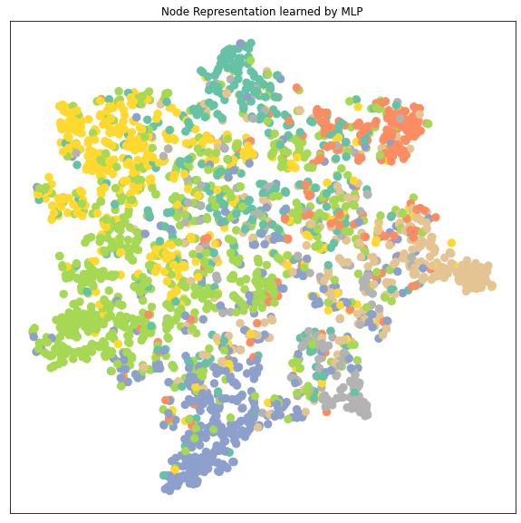
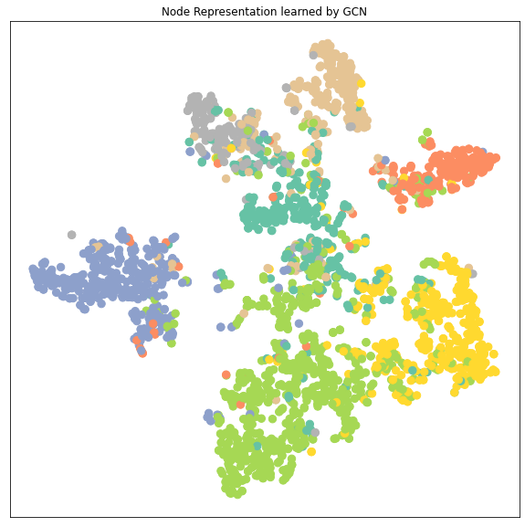
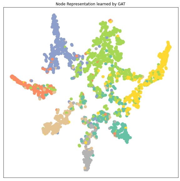
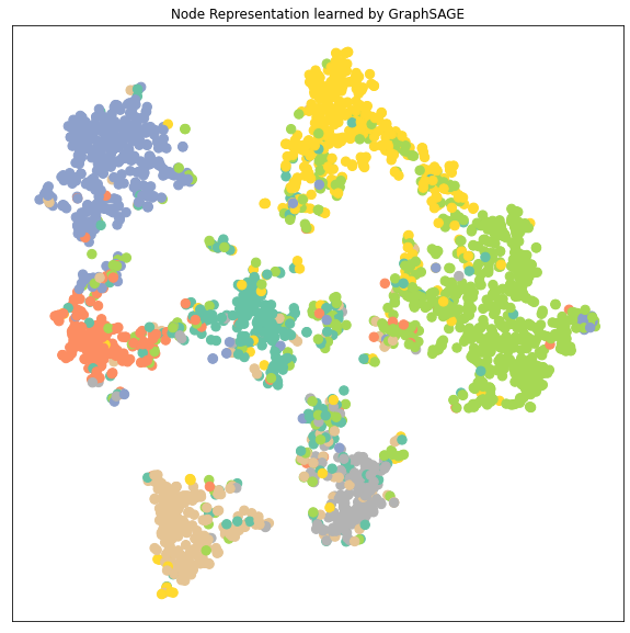
从降维后的 node embedding的cluster的分布来分析不同模型的性能:
- 可以看到GCN, GAT, GraphSAGE 的node embedding的7个clusters都比MLP要区分得清楚,即每个类的特征差异较大容易被识别出来所以GNN都比MLP要好
- GAT和GraphSAGE的clusters之间的距离都比GCN的clusters之间的距离要远,特别是GAT。GAT的每个cluster都收缩成一束一束的聚合起来。而因为这里显示的cluster是data.x样本,包括了训练集在内,所以cluster区分得越明显很有可能是数据拟合得很好甚至是有overfitting的可能。
1 |
4. Assignment
- 此篇文章涉及的代码可见于
codes/learn_node_representation.ipynb,请参照这份代码使用PyG中不同的图卷积模块在PyG的不同数据集上实现节点分类或回归任务。
4.1 Dataset选择
- Pubmed: https://arxiv.org/abs/1603.08861
这个数据集合Cora一样: Nodes represent documents and edges represent citation links - Citeseer: https://arxiv.org/abs/1603.08861
这个数据集合Cora一样: Nodes represent documents and edges represent citation links - CitationFull: https://arxiv.org/abs/1707.03815
Nodes represent documents and edges represent citation links. - 本来想尝试其他数据,但是其他数据集太大训练起来很慢,后期有时间再试试看
这里写个函数一次性打印所有要用的dataset的信息,看一下不同dataset的node, edge信息,并用table打印出来
1 | # dataset used by GAT |
Downloading https://data.dgl.ai/dataset/ppi.zip
Extracting dataset/ppi.zip
1 | import pandas as pd |
dataset:  CitationFull
dataset:  Pubmed
dataset:  Citeseer
| 0 | 1 | 2 | |
|---|---|---|---|
| dataset | CitationFull | Pubmed | Citeseer |
| #graphs | 1 | 1 | 1 |
| #features | 1639 | 500 | 3703 |
| #classes | 4 | 3 | 6 |
| #nodes | 17716 | 19717 | 3327 |
| #edges | 105734 | 88648 | 9104 |
| Has_isolated_nodes | False | False | True |
| undirected | True | True | True |
1 | # KarateClub_dataset[0] |
4.2 GNN Model Training
这里写个一次性训练所有模型和训练集的函数,并把所有模型的结果打印
1 | models = {} |
1 | test_results, trained_models = train_models(models, mydatasets) |
Dataset: CitationFull, model: MLP
Epoch: 020, Loss: 0.9961
Epoch: 040, Loss: 0.8182
Epoch: 060, Loss: 0.7515
Epoch: 080, Loss: 0.7192
Epoch: 100, Loss: 0.6986
Epoch: 120, Loss: 0.6905
Epoch: 140, Loss: 0.6799
Epoch: 160, Loss: 0.6746
Epoch: 180, Loss: 0.6669
Epoch: 200, Loss: 0.6673

Test Accuracy: 0.8128
Dataset: CitationFull, model: GCN
Epoch: 020, Loss: 0.7686
Epoch: 040, Loss: 0.5725
Epoch: 060, Loss: 0.5072
Epoch: 080, Loss: 0.4807
Epoch: 100, Loss: 0.4712
Epoch: 120, Loss: 0.4601
Epoch: 140, Loss: 0.4548
Epoch: 160, Loss: 0.4475
Epoch: 180, Loss: 0.4489
Epoch: 200, Loss: 0.4439

Test Accuracy: 0.8606
Dataset: CitationFull, model: GAT
Epoch: 020, Loss: 0.7240
Epoch: 040, Loss: 0.5830
Epoch: 060, Loss: 0.4896
Epoch: 080, Loss: 0.4724
Epoch: 100, Loss: 0.4547
Epoch: 120, Loss: 0.4440
Epoch: 140, Loss: 0.4313
Epoch: 160, Loss: 0.4150
Epoch: 180, Loss: 0.4025
Epoch: 200, Loss: 0.3877

Test Accuracy: 0.8818
Dataset: CitationFull, model: GraphSAGE
Epoch: 020, Loss: 0.4138
Epoch: 040, Loss: 0.2719
Epoch: 060, Loss: 0.2323
Epoch: 080, Loss: 0.2151
Epoch: 100, Loss: 0.2272
Epoch: 120, Loss: 0.1943
Epoch: 140, Loss: 0.2020
Epoch: 160, Loss: 0.1900
Epoch: 180, Loss: 0.1968
Epoch: 200, Loss: 0.2002

Test Accuracy: 0.9690
Dataset: Pubmed, model: MLP
Epoch: 020, Loss: 0.4589
Epoch: 040, Loss: 0.1964
Epoch: 060, Loss: 0.1649
Epoch: 080, Loss: 0.1044
Epoch: 100, Loss: 0.0887
Epoch: 120, Loss: 0.1578
Epoch: 140, Loss: 0.1371
Epoch: 160, Loss: 0.1269
Epoch: 180, Loss: 0.1296
Epoch: 200, Loss: 0.1131

Test Accuracy: 0.7280
Dataset: Pubmed, model: GCN
Epoch: 020, Loss: 0.5874
Epoch: 040, Loss: 0.2958
Epoch: 060, Loss: 0.2396
Epoch: 080, Loss: 0.1658
Epoch: 100, Loss: 0.1735
Epoch: 120, Loss: 0.1848
Epoch: 140, Loss: 0.1198
Epoch: 160, Loss: 0.1091
Epoch: 180, Loss: 0.1549
Epoch: 200, Loss: 0.1069

Test Accuracy: 0.7930
Dataset: Pubmed, model: GAT
Epoch: 020, Loss: 0.3768
Epoch: 040, Loss: 0.1317
Epoch: 060, Loss: 0.1555
Epoch: 080, Loss: 0.2786
Epoch: 100, Loss: 0.1570
Epoch: 120, Loss: 0.1774
Epoch: 140, Loss: 0.0932
Epoch: 160, Loss: 0.1104
Epoch: 180, Loss: 0.0623
Epoch: 200, Loss: 0.0201

Test Accuracy: 0.7140
Dataset: Pubmed, model: GraphSAGE
Epoch: 020, Loss: 0.0753
Epoch: 040, Loss: 0.0226
Epoch: 060, Loss: 0.0557
Epoch: 080, Loss: 0.0116
Epoch: 100, Loss: 0.0086
Epoch: 120, Loss: 0.0297
Epoch: 140, Loss: 0.0106
Epoch: 160, Loss: 0.0835
Epoch: 180, Loss: 0.0064
Epoch: 200, Loss: 0.0906

Test Accuracy: 0.7700
Dataset: Citeseer, model: MLP
Epoch: 020, Loss: 1.1613
Epoch: 040, Loss: 0.5621
Epoch: 060, Loss: 0.4475
Epoch: 080, Loss: 0.4112
Epoch: 100, Loss: 0.3795
Epoch: 120, Loss: 0.3416
Epoch: 140, Loss: 0.3785
Epoch: 160, Loss: 0.3341
Epoch: 180, Loss: 0.3596
Epoch: 200, Loss: 0.4045

Test Accuracy: 0.5910
Dataset: Citeseer, model: GCN
Epoch: 020, Loss: 1.3142
Epoch: 040, Loss: 0.8198
Epoch: 060, Loss: 0.5696
Epoch: 080, Loss: 0.4871
Epoch: 100, Loss: 0.4850
Epoch: 120, Loss: 0.4268
Epoch: 140, Loss: 0.3961
Epoch: 160, Loss: 0.3845
Epoch: 180, Loss: 0.3508
Epoch: 200, Loss: 0.3517

Test Accuracy: 0.7010
Dataset: Citeseer, model: GAT
Epoch: 020, Loss: 0.7527
Epoch: 040, Loss: 0.4082
Epoch: 060, Loss: 0.4495
Epoch: 080, Loss: 0.4963
Epoch: 100, Loss: 0.3861
Epoch: 120, Loss: 0.2898
Epoch: 140, Loss: 0.3495
Epoch: 160, Loss: 0.2082
Epoch: 180, Loss: 0.2877
Epoch: 200, Loss: 0.3382

Test Accuracy: 0.6530
Dataset: Citeseer, model: GraphSAGE
Epoch: 020, Loss: 0.3369
Epoch: 040, Loss: 0.1300
Epoch: 060, Loss: 0.0721
Epoch: 080, Loss: 0.0956
Epoch: 100, Loss: 0.1785
Epoch: 120, Loss: 0.0476
Epoch: 140, Loss: 0.0424
Epoch: 160, Loss: 0.0556
Epoch: 180, Loss: 0.1063
Epoch: 200, Loss: 0.0645

Test Accuracy: 0.6720
| CitationFull | Pubmed | Citeseer | |
|---|---|---|---|
| MLP | 0.812768 | 0.728 | 0.591 |
| GCN | 0.860634 | 0.793 | 0.701 |
| GAT | 0.881802 | 0.714 | 0.653 |
| GraphSAGE | 0.969011 | 0.770 | 0.672 |
Conclusion
- 和以往的像图片文本之类的数据不同,图的数据的训练的不同点有下面几个
- 除了要输入节点的数据特征外,还要输入edge作为关联的数据。
- 另外GNN在训练时是可以同时更新多个不同node的embedding。
- GNN训练时更加像NLP的训练方法,都是把一部分的node(在NLP里面是word token)mask掉并对这部分内容(node或者link)预测
- 另外在node classification里面因为GNN输入是图,输出也是转换后学习后的图(图里的每个node的值代表这个node所属的class),可以一下子把所有要预测的node进行预测。不过也可以通过mask的形式在图里面采样进行分batch训练
- 另外在上面实验中可以看到,在相同配置中GCN要把GAT和GraphSAGE好,GAT比较容易overfit,而GAT和GraphSAGE训练相对于GCN比较慢因为在训练node embedding时设计到两个循环。不过GAT,GraphSAGE相对于GCN训练时的loss收敛得很快。就目前的任务来看感觉GCN比GAT,GraphSAGE要好,但是可能不同的任务模型用起来效果也不一样
- 当node embedding训练得好的时候,不同的类的node embedding特征很容易被区别开来,相同类的node的特征会内聚而不同类的特征会远离,这个其实和普通的NN分类器里面提取的特征一样,比较正常。
Reference
- Datawhale:https://github.com/datawhalechina/team-learning-nlp/blob/master/GNN/Markdown%E7%89%88%E6%9C%AC/5-%E5%9F%BA%E4%BA%8E%E5%9B%BE%E7%A5%9E%E7%BB%8F%E7%BD%91%E7%BB%9C%E7%9A%84%E8%8A%82%E7%82%B9%E8%A1%A8%E5%BE%81%E5%AD%A6%E4%B9%A0.md
- 知乎 https://zhuanlan.zhihu.com/p/106706203
- PyG中内置的数据转换方法:torch-geometric-transforms
- 一个可视化高纬数据的工具:t-distributed Stochastic Neighbor Embedding
- 提出GCN的论文:Semi-supervised Classification with Graph Convolutional Network
- GCNConv官方文档:torch_geometric.nn.conv.GCNConv
- 提出GAT的论文: Graph Attention Networks