GNN-5-ClusterGCN
GCN-Task-5-Cluster GCN
1. Introduction
这篇文章的目的主要是理解 Cluster-GCN这篇文章的内容(要解决的问题,思路,等)和通过代码实现一下Cluster-GCN网络。 Cluster-GCN的文章可以查看: https://arxiv.org/pdf/1905.07953.pdf
这篇blog的结构大概如下:
- 解释Cluster-GCN的内容
- Cluster-GCN要解决的问题
- 基本思路
- Cluster-GCN的特点和优缺点
- Coding实现
- 数据集
- Cluster-GCN模型
- Training and Testing
- Assignment from datawhale
- 总结文章的重点
- Reference 参考文献
2. Cluster-GCN
Cluster GCN是由国立台湾大学Wei-Lin Chiang,Google research 的Yang Li和 Samy Bengio, Cho-Jui Hsieh 等人提出的GCN网络(看到Bengio等Google大牛的名字就知道这篇文章很值得一读)。文章的全称是Cluster-GCN: An Efficient Algorithm for Training Deep and Large Graph Convolutional Networks。 从名字就可以知道这个Cluster-GCN的目的是要优化深度学习和超大图网络的效率而提出来的(一般都会涉及时间和空间的复杂度分析)。这里先来看看这篇文章要解决的问题
2.1 Problem to solve
首先这篇文章提出和分析了在GNN学习里面的几个问题:
Full-batch gradient descent:
这里先做以下定义
node的个数为N
Embedding dimension = F
GCN的layer层数为L.
那么在用Full batch GD 全梯度下降方法时所需的Space Complexity = O(NFL)并且计算梯度时如果node个数很多有上百万个,每个epoch里面梯度计算也是很慢的。因此这种方法不考虑
Mini-batch SGD
Mini-batch SGD算是对Full batch GD的方法通过随机采样降低要计算的梯度的存储空间以及加快了计算的速度。 但是mini-batch SGD会使得时间复杂度随着GCN的层数增加而指数级增长。paper原话是这么解释的:
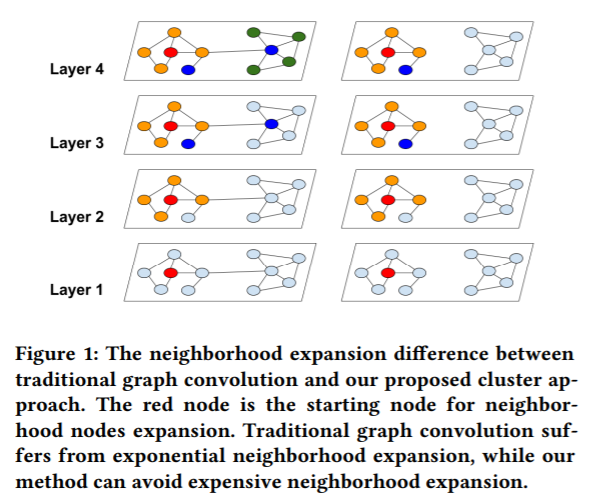
mini-batch SGD introduces a significant computational overhead due to the neighborhood expansion problem—to compute the loss on a single node at layer L, it requires that node’s neighbor nodes’ embeddings at layer L − 1, which again requires their neighbors’ embeddings at layer L − 2 and recursive ones in the downstream layers. This leads to time complexity exponential to the GCN depth.
用我自己的话来理解就是,以下图为例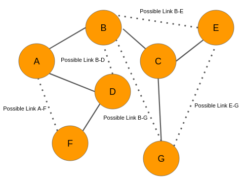
如果在GCN第i层的第j个节点的embedding vector用$Z_ {i}^{j}$,而第i个节点的neighbor用$N(i)$表示, 那么在第0层输入层节点A的embedding就是$Z_ {A}^{0}$, $N(A)$ = {B,D}。那么我们就有以下的公式:- 在第1层 L1, $Z_ {A}^{1} = f(Z_ {B}^{0}, Z_ {D}^{0}, Z_ {A}^{0})$
- 在第2层 L2, $Z_ {A}^{2} = f(Z_ {B}^{1}, Z_ {D}^{1}, Z_ {A}^{1})$, 而其中又可以把$Z_ {A}^{1}$ 展开成L1层里面的式子,$Z_ {B}^{1},Z_ {D}^{1}$ 同理
- 第3层L3, $Z_ {A}^{3} = f(Z_ {B}^{2}, Z_ {D}^{2}, Z_ {A}^{2})$, 计算时和第二步同理可以多次展开成用L1层的输入表示的形式,这么一来可以看到,随着GCN层数增加,neighborhood expansion problem 邻居展开问题就会使得梯度计算更加复杂
- 这个节点i在第j层梯度计算都取决于第j-1层前面一层的计算就是neighborhood expansion problem
- 如果GCN层数为L, 节点的平均degree为d,那么我们计算一个节点的梯度就需要$O(d ^L)$个节点embedding信息, 而由于要乘上权重矩阵W, 计算每个node的embedding需要O($F^2$) 的时间。 那么计算一个node的梯度为$O(d ^LF^2)$
- VR-GCN(variance reduction GCN), it uses variance reduction technique to reduce the size of neighborhood sampling nodes
2.2 How Cluster-GCN works
2.2.1 Cluster-GCN的思想
ClusterGCN的想法是我们能不能找到一把种将节点分成多个batch的方式,并将图划分成多个子图,使得表征利用率最大?我们通过将表征利用率的概念与图节点聚类的目标联系起来来回答这个问题。原文:can we design a batch and the corresponding computation subgraph to maximize the embedding utilization?
节点表征的利用率可以反映出计算的效率。考虑到一个batch有多个节点,时间与空间复杂度的计算就不是上面那样简单了,因为不同的节点同样距离远的邻接节点可以是重叠的,于是计算表征的次数可以小于最坏的情况$O(b d^{L})$。为了反映mini-batch SGD的计算效率,Cluster-GCN论文提出了**”表征利用率”的概念来描述计算效率。在训练过程中,如果节点$i$在$l$层的表征$z_{i}^{(l)}$被计算并在$l+1$层的表征计算中被重复使用$u$次,那么我们说$z_{i}^{(l)}$的表征利用率为$u$。对于随机抽样的mini-batch SGD,$u$非常小,因为图通常是大且稀疏的。假设$u$是一个小常数(节点间同样距离的邻接节点重叠率小),那么mini-batch SGD的训练方式对每个batch需要计算$O(b d^{L})$的表征,于是每次参数更新需要$O(b d^{L} F^{2})$的时间,每个epoch需要$O(N d^{L} F^{2})$的时间,这被称为邻域扩展问题**。
相反的是,全梯度下降训练具有最大的表征利用率——每个节点表征将在上一层被重复使用平均节点度次。因此,全梯度下降法在每个epoch中只需要计算$O(N L)$的表征,这意味着平均下来只需要$O(L)$的表征计算就可以获得一个节点的梯度。
2.2.2 简单的Cluster-GCN方法
考虑到在每个batch中,我们计算一组节点(记为$\mathcal{B}$)从第$1$层到第$L$层的表征。由于图神经网络每一层的计算都使用相同的子图$A_{\mathcal{B}, \mathcal{B}}$($\mathcal{B}$内部的边),所以表征利用率就是这个batch内边的数量,记为$|A_{\mathcal{B}, \mathcal{B}}|_{0}$。因此,为了最大限度地提高表征利用率,理想的划分batch的结果是,batch内的边尽可能多,batch之间的边尽可能少。基于这一点,我们将SGD图神经网络训练的效率与图聚类算法联系起来。
现在我们正式学习Cluster-GCN方法。对于一个图$G$,我们将其节点划分为$c$个簇:$\mathcal{V}=[\mathcal{V}_ {1}, \cdots \mathcal{V}_ {c}]$,其中$\mathcal{V}{t}$由第$t$个簇中的节点组成,对应的我们有$c$个子图:
$$
\bar{G}=[G{1}, \cdots, G_{c}]=[{\mathcal{V}_ {1}, \mathcal{E}_ {1}}, \cdots,{\mathcal{V}_ {c}, \mathcal{E}_ {c}}]
\notag
$$
其中$\mathcal{E}{t}$只由$\mathcal{V}{t}$中的节点之间的边组成。经过节点重组,邻接矩阵被划分为大小为$c^{2}$的块矩阵,如下所示
$$
A=\bar{A}+\Delta=[\begin{array}{ccc}
A_{11} & \cdots & A_{1 c} \\
\vdots & \ddots & \vdots \\
A_{c 1} & \cdots & A_{c c}
\end{array}]
\tag{4}
$$
其中
$$
\bar{A}=[\begin{array}{ccc}
A_{11} & \cdots & 0 \\
\vdots & \ddots & \vdots \\
0 & \cdots & A_{c c}
\end{array}], \Delta=[\begin{array}{ccc}
0 & \cdots & A_ {1 c} \\
\vdots & \ddots & \vdots \\
A_{c 1} & \cdots & 0
\end{array}]
\tag{5}
$$
其中,对角线上的块$A_{t t}$是大小为$|\mathcal{V}{t}| \times|\mathcal{V}{t}|$的邻接矩阵,它由$G_{t}$内部的边构成。$\bar{A}$是图$\bar{G}$的邻接矩阵。$A_{s t}$由两个簇$\mathcal{V}_ {s}$和$\mathcal{V}_ {t}$之间的边构成。$\Delta$是由$A$的所有非对角线块组成的矩阵。同样,我们可以根据$[\mathcal{V}_ {1}, \cdots, \mathcal{V}_ {c}]$ 划分节点表征矩阵$X$和类别向量 $Y$,得到$[X_{1}, \cdots, X_{c}]$和$[Y_{1}, \cdots, Y_{c}]$,其中$X_{t}$和$Y_{t}$分别由$V_{t}$中节点的表征和类别组成。
接下来我们用块对角线邻接矩阵 $\bar{A}$ 去近似邻接矩阵$A$,这样做的好处是,完整的损失函数(公示(2))可以根据batch分解成多个部分之和。以$\bar{A}^{\prime}$表示归一化后的$\bar{A}$,最后一层节点表征矩阵可以做如下的分解:
$$
\begin{aligned}
Z^{(L)} &=\bar{A}^{\prime} \sigma(\bar{A}^{\prime} \sigma(\cdots \sigma(\bar{A}^{\prime} X W^{(0)}) W^{(1)}) \cdots) W^{(L-1)} \\
&=[\begin{array}{c}
\bar{A}_ {11}^{\prime} \sigma(\bar{A}_ {11}^{\prime} \sigma(\cdots \sigma(\bar{A}_ {11}^{\prime} X_{1} W^{(0)}) W^{(1)}) \cdots) W^{(L-1)} \\
\vdots \\
\bar{A}_ {c c}^{\prime} \sigma(\bar{A}_ {c c}^{\prime} \sigma(\cdots \sigma(\bar{A}_ {c c}^{\prime} X_{c} W^{(0)}) W^{(1)}) \cdots) W^{(L-1)}
\end{array}]
\end{aligned}
\tag{6}
$$
由于$\bar{A}$是块对角形式($\bar{A}_ {t t}^{\prime}$是$\bar{A}^{\prime}$的对角线上的块),于是损失函数可以分解为
$$
\mathcal{L}_ {\bar{A}^{\prime}}=\sum_{t} \frac{|\mathcal{V}_ {t}|}{N} \mathcal{L}_ {\bar{A}_ {t t}^{\prime}} \text { and } \mathcal{L}_ {\bar{A}_ {t t}^{\prime}}=\frac{1}{|\mathcal{V}_ {t}|} \sum_{i \in \mathcal{V}_ {t}} \operatorname{loss}(y_{i}, z_{i}^{(L)})
\tag{7}
$$
基于公式(6)和公式(7),在训练的每一步中,Cluster-GCN首先采样一个簇 $\mathcal{V}_ {t}$,然后根据$\mathcal{L}_ {\bar{A}^{\prime}_ {tt}}$ 的梯度进行参数更新。这种训练方式,只需要用到子图 $A_{t t}$, $X_{t}$, $Y_{t}$ 以及神经网络权重矩阵 ${W^{(l)}}_{l=1}^{L}$。 实际中,主要的计算开销在神经网络前向过程中的矩阵乘法运算(公式(6)的一个行)和梯度反向传播。
我们使用图节点聚类算法来划分图。图节点聚类算法将图节点分成多个簇,划分结果是簇内边的数量远多于簇间边的数量。如前所述,每个batch的表征利用率相当于簇内边的数量。直观地说,每个节点和它的邻接节点大部分情况下都位于同一个簇中,因此 $L$ 跳(L-hop)远的邻接节点大概率仍然在同一个簇中。由于我们用块对角线近似邻接矩阵$\bar{A}$代替邻接矩阵$A$,产生的误差与簇间的边的数量$\Delta$成正比,所以簇间的边越少越好。综上所述,使用图节点聚类算法对图节点划分多个簇的结果,正是我们希望得到的。
在下图,我们可以看到,Cluster-GCN方法可以避免巨大范围的邻域扩展(图右),因为Cluster-GCN方法将邻域扩展限制在簇内。
2.2.3 Cluster-GCN实现过程

从上图可以看到, Cluster-GCN的实现流程基本是
- 用METIS partition算法对图的节点进行分解成c个cluster
- 不断迭代, 每次迭代都随机选取q个cluster进行无放回采样node,links并形成subgraph
- 对subgraph进行预测和gradient计算
- 用adam进行node的更新和学习
另外 Cluster-GCN方法提出了一个修改版的公式(9),以更好地保持邻接节点信息和数值范围。首先给原始的$A$添加一个单位矩阵$I$,并进行归一化处理
$$
\tilde{A}=(D+I)^{-1}(A+I)
\tag{10}
$$
然后考虑,
$$
X^{(l+1)}=\sigma((\tilde{A}+\lambda \operatorname{diag}(\tilde{A})) X^{(l)} W^{(l)})
\tag{11}
$$
以上就是Cluster-GCN的每层layer的更新输出公式
2.3 Properties
- Advantage
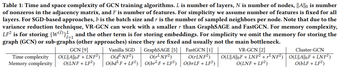
先来看看时间和空间复杂度。 在时间上它只和layer层数 L, embedding feature的大小F以及邻接矩阵的非零的行数||A||和节点个数有关, 而空间上和batch的大小相关,相对于传统的GCN,它把指数次降到1次
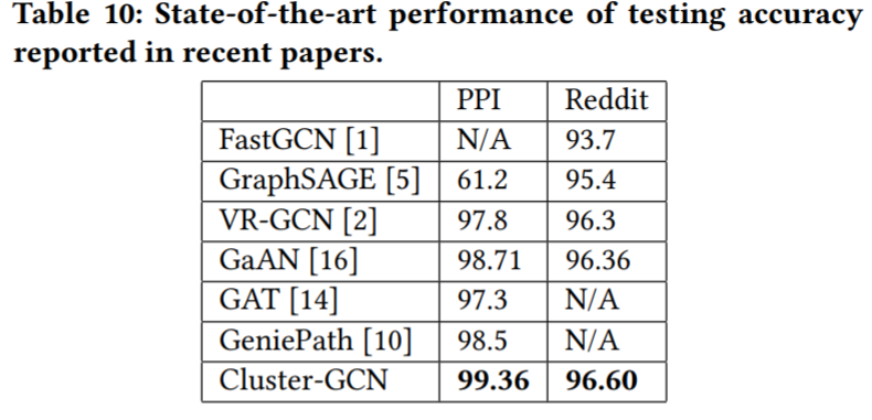
除了Time, Space complexity外, paper里面提及在大型的图数据里面如PPI, Reddit是最好的(这个可能有调参的因素在里面)
- Shortage
- 在收敛性上面, Cluster-GCN在layer数量超过3层之后Accuracy性能没有明显变大,反而layer到了6层之后,开始收敛不好性能变差,如下图所示
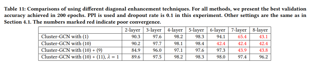
- 在收敛性上面, Cluster-GCN在layer数量超过3层之后Accuracy性能没有明显变大,反而layer到了6层之后,开始收敛不好性能变差,如下图所示
- Other properties
- ClusterGCN在做clustering对节点进行cluster partition时特意对比了 random partition和METIS clustering partition两种方法, 以及batch设计时是用多个cluster还是一个cluster作为一个batch。它表明了用METIS和 multiple clusters as a batch 更能使性能提升,loss降低更多。
1 |
1 |
1 |
1 |
3.1 官方测试源码
这里用了Reddit的dataset进行测试
1 | import torch |
Downloading https://data.dgl.ai/dataset/reddit.zip
Extracting data/Reddit/raw/reddit.zip
Processing...
Done!
Computing METIS partitioning...
Done!


/home/wenkanw/.conda/envs/mlenv/lib/python3.8/site-packages/torch/utils/data/dataloader.py:474: UserWarning: This DataLoader will create 12 worker processes in total. Our suggested max number of worker in current system is 8, which is smaller than what this DataLoader is going to create. Please be aware that excessive worker creation might get DataLoader running slow or even freeze, lower the worker number to avoid potential slowness/freeze if necessary.
  warnings.warn(_create_warning_msg(


Epoch: 01, Loss: 1.0684
Epoch: 02, Loss: 0.4532
Epoch: 03, Loss: 0.3874
Epoch: 04, Loss: 0.3552


Evaluating: 100%|██████████| 465930/465930 [00:42<00:00, 10886.52it/s]

Epoch: 05, Loss: 0.3361, Train: 0.9568, Val: 0.9523, test: 0.9509


Epoch: 06, Loss: 0.3220
Epoch: 07, Loss: 0.3259
Epoch: 08, Loss: 0.3068
Epoch: 09, Loss: 0.2899


Evaluating: 100%|██████████| 465930/465930 [00:43<00:00, 10825.21it/s]

Epoch: 10, Loss: 0.2844, Train: 0.9639, Val: 0.9517, test: 0.9523


Epoch: 11, Loss: 0.2850
Epoch: 12, Loss: 0.2700
Epoch: 13, Loss: 0.2705
Epoch: 14, Loss: 0.2696


Evaluating: 100%|██████████| 465930/465930 [00:43<00:00, 10803.24it/s]

Epoch: 15, Loss: 0.2793, Train: 0.9637, Val: 0.9524, test: 0.9506


Epoch: 16, Loss: 0.2699
Epoch: 17, Loss: 0.2556
Epoch: 18, Loss: 0.2656
Epoch: 19, Loss: 0.2642


Evaluating: 100%|██████████| 465930/465930 [00:43<00:00, 10797.29it/s]


Epoch: 20, Loss: 0.2491, Train: 0.9686, Val: 0.9551, test: 0.9537
Epoch: 21, Loss: 0.2450
Epoch: 22, Loss: 0.2449
Epoch: 23, Loss: 0.2456
Epoch: 24, Loss: 0.2491


Evaluating: 100%|██████████| 465930/465930 [00:43<00:00, 10737.69it/s]


Epoch: 25, Loss: 0.2518, Train: 0.9572, Val: 0.9433, test: 0.9389
Epoch: 26, Loss: 0.2430
Epoch: 27, Loss: 0.2342
Epoch: 28, Loss: 0.2297
Epoch: 29, Loss: 0.2270


Evaluating: 100%|██████████| 465930/465930 [00:43<00:00, 10824.00it/s]


Epoch: 30, Loss: 0.2319, Train: 0.9716, Val: 0.9514, test: 0.9517
3.2 自己调整的代码
1 | import os |
1
41
232965
114615892
602
1 | class ClusterGCNNet(torch.nn.Module): |
1 |
|
1 |
1 | import torch |
Using num cluster: 500
Partition Time: 1.7125461101531982 s

Epoch: 01, Loss: 1.8346
Epoch: 02, Loss: 0.6928
Epoch: 03, Loss: 0.4838
Epoch: 04, Loss: 0.4009


Evaluating: 100%|██████████| 465930/465930 [00:57<00:00, 8127.96it/s]

Epoch: 05, Loss: 0.3632, Train: 0.9541, Val: 0.9542, test: 0.9531

Epoch: 06, Loss: 0.3425
Epoch: 07, Loss: 0.3161
Epoch: 08, Loss: 0.3140
Epoch: 09, Loss: 0.3006

Evaluating: 100%|██████████| 465930/465930 [00:56<00:00, 8212.24it/s]

Epoch: 10, Loss: 0.2787, Train: 0.9637, Val: 0.9586, test: 0.9571

Epoch: 11, Loss: 0.2684
Epoch: 12, Loss: 0.2558
Epoch: 13, Loss: 0.2522
Epoch: 14, Loss: 0.2455


Evaluating: 100%|██████████| 465930/465930 [01:00<00:00, 7730.12it/s]

Epoch: 15, Loss: 0.2421, Train: 0.9667, Val: 0.9577, test: 0.9565

Epoch: 16, Loss: 0.2649
Epoch: 17, Loss: 0.2377
Epoch: 18, Loss: 0.2277
Epoch: 19, Loss: 0.2190

Evaluating: 100%|██████████| 465930/465930 [00:54<00:00, 8495.90it/s]

Epoch: 20, Loss: 0.2151, Train: 0.9698, Val: 0.9568, test: 0.9559

Epoch: 21, Loss: 0.2138
Epoch: 22, Loss: 0.2101
Epoch: 23, Loss: 0.2084
Epoch: 24, Loss: 0.2062

Evaluating: 100%|██████████| 465930/465930 [00:58<00:00, 7914.75it/s]

Epoch: 25, Loss: 0.2057, Train: 0.9713, Val: 0.9558, test: 0.9545

Epoch: 26, Loss: 0.2061
Epoch: 27, Loss: 0.2097
Epoch: 28, Loss: 0.2099
Epoch: 29, Loss: 0.2035

Evaluating: 100%|██████████| 465930/465930 [00:59<00:00, 7891.56it/s]

Epoch: 30, Loss: 0.1938, Train: 0.9736, Val: 0.9567, test: 0.9560
Training Time: 0:09:43.498993 s
Using num cluster: 1000
Partition Time: 3.144443988800049 s
Epoch: 01, Loss: 1.4359
Epoch: 02, Loss: 0.5340
Epoch: 03, Loss: 0.4172
Epoch: 04, Loss: 0.3630

Evaluating: 100%|██████████| 465930/465930 [00:58<00:00, 7984.94it/s]

Epoch: 05, Loss: 0.3458, Train: 0.9358, Val: 0.9350, test: 0.9327

Epoch: 06, Loss: 0.3326
Epoch: 07, Loss: 0.3068
Epoch: 08, Loss: 0.2879
Epoch: 09, Loss: 0.2861

Evaluating: 100%|██████████| 465930/465930 [00:59<00:00, 7885.83it/s]

Epoch: 10, Loss: 0.2757, Train: 0.9618, Val: 0.9536, test: 0.9506
Epoch: 11, Loss: 0.2700
Epoch: 12, Loss: 0.2535
Epoch: 13, Loss: 0.2523
Epoch: 14, Loss: 0.2461

Evaluating: 100%|██████████| 465930/465930 [00:59<00:00, 7813.02it/s]

Epoch: 15, Loss: 0.2412, Train: 0.9688, Val: 0.9568, test: 0.9548

Epoch: 16, Loss: 0.2470
Epoch: 17, Loss: 0.2456
Epoch: 18, Loss: 0.2403
Epoch: 19, Loss: 0.2296

Evaluating: 100%|██████████| 465930/465930 [00:54<00:00, 8482.81it/s]

Epoch: 20, Loss: 0.2284, Train: 0.9696, Val: 0.9546, test: 0.9545

Epoch: 21, Loss: 0.2276
Epoch: 22, Loss: 0.2219
Epoch: 23, Loss: 0.2224
Epoch: 24, Loss: 0.2233

Evaluating: 100%|██████████| 465930/465930 [00:57<00:00, 8037.32it/s]

Epoch: 25, Loss: 0.2241, Train: 0.9698, Val: 0.9533, test: 0.9520

Epoch: 26, Loss: 0.2226
Epoch: 27, Loss: 0.2129
Epoch: 28, Loss: 0.2171
Epoch: 29, Loss: 0.2312

Evaluating: 100%|██████████| 465930/465930 [00:58<00:00, 7972.01it/s]

Epoch: 30, Loss: 0.2149, Train: 0.9739, Val: 0.9559, test: 0.9539
Training Time: 0:09:46.712217 s
Using num cluster: 1500
Partition Time: 1.5299558639526367 s
Epoch: 01, Loss: 1.1529
Epoch: 02, Loss: 0.4863
Epoch: 03, Loss: 0.3942
Epoch: 04, Loss: 0.3567

Evaluating: 100%|██████████| 465930/465930 [01:00<00:00, 7716.31it/s]

Epoch: 05, Loss: 0.3439, Train: 0.9559, Val: 0.9524, test: 0.9513

Epoch: 06, Loss: 0.3230
Epoch: 07, Loss: 0.3062
Epoch: 08, Loss: 0.3013
Epoch: 09, Loss: 0.3049

Evaluating: 100%|██████████| 465930/465930 [01:00<00:00, 7741.65it/s]

Epoch: 10, Loss: 0.2984, Train: 0.9609, Val: 0.9518, test: 0.9501

Epoch: 11, Loss: 0.2839
Epoch: 12, Loss: 0.2775
Epoch: 13, Loss: 0.2720
Epoch: 14, Loss: 0.2701

Evaluating: 100%|██████████| 465930/465930 [01:01<00:00, 7567.86it/s]

Epoch: 15, Loss: 0.2634, Train: 0.9633, Val: 0.9513, test: 0.9495

Epoch: 16, Loss: 0.2851
Epoch: 17, Loss: 0.2721
Epoch: 18, Loss: 0.2635
Epoch: 19, Loss: 0.2489

Evaluating: 100%|██████████| 465930/465930 [01:00<00:00, 7680.40it/s]

Epoch: 20, Loss: 0.2617, Train: 0.9645, Val: 0.9495, test: 0.9494

Epoch: 21, Loss: 0.2517
Epoch: 22, Loss: 0.2424
Epoch: 23, Loss: 0.2411
Epoch: 24, Loss: 0.2370

Evaluating: 100%|██████████| 465930/465930 [01:00<00:00, 7762.74it/s]

Epoch: 25, Loss: 0.2379, Train: 0.9702, Val: 0.9521, test: 0.9517

Epoch: 26, Loss: 0.2414
Epoch: 27, Loss: 0.2358
Epoch: 28, Loss: 0.2325
Epoch: 29, Loss: 0.2406

Evaluating: 100%|██████████| 465930/465930 [01:00<00:00, 7753.34it/s]

Epoch: 30, Loss: 0.2327, Train: 0.9633, Val: 0.9450, test: 0.9433
Training Time: 0:10:01.358439 s
Using num cluster: 2000
Computing METIS partitioning...
Done!
Partition Time: 298.0074031352997 s
3.3 Result
这里因为训练时我尝试了不同的cluster的数目,但是都是试了3种不同cluster数目之后就内存溢出,所以这里我尝试跑了2次,分别对比500,1000,1500以及1000,1500,2000两种情况。可以看到随着cluster数目的增多 test accuracy的的变化是先大后小,而且变化的幅度不大一般都在1%左右
1 | df_result = pd.DataFrame(result) |
| num_cluster | partition_t | train_t | train_acc | val_acc | test_acc | |
|---|---|---|---|---|---|---|
| 0 | 500 | 1.712546 | 0 days 00:09:43.498993 | 0.973591 | 0.956695 | 0.955999 |
| 1 | 1000 | 3.144444 | 0 days 00:09:46.712217 | 0.973949 | 0.955898 | 0.953916 |
| 2 | 1500 | 1.529956 | 0 days 00:10:01.358439 | 0.963299 | 0.945030 | 0.943306 |
1 | pd.DataFrame(result) |
| num_cluster | partition_t | train_t | train_acc | val_acc | test_acc | |
|---|---|---|---|---|---|---|
| 0 | 2000 | 2.519914 | 0 days 00:04:56.476637 | 0.966519 | 0.948219 | 0.947866 |
| 1 | 1500 | 3.753822 | 0 days 00:06:28.267962 | 0.971231 | 0.953674 | 0.952803 |
| 2 | 1000 | 2.336999 | 0 days 00:07:26.611871 | 0.971479 | 0.951534 | 0.950075 |
4. Conclusion and Take-away
ClusterGCN的成果
- 对不同的batch,graph partition的方法进行研究
- 通过batch的设计和Clustering partition(METIS) 对GCN算法的Time, Space Complexity 在大型图数据里面有很大的提升(解决了neighborhood expansion problem问题)
- 相对于VR-GCN, 训练时间随着DNN 层数变多而增加的幅度不大。 Cluster-GCN的训练时间随着层数增多几乎是线性的。
- 能够用于训练大型embedding的特征
Note
- Vanilla 在CS里面的含义
vanilla is the term used to refer when computer software and sometimes also other computing-related systems like computer hardware or algorithms are not customized from their original form
- Vanilla 在CS里面的含义
5. Reference
[1] Datawhale: https://github.com/datawhalechina/team-learning-nlp/blob/master/GNN/Markdown%E7%89%88%E6%9C%AC/7-%E8%B6%85%E5%A4%A7%E5%9B%BE%E4%B8%8A%E7%9A%84%E8%8A%82%E7%82%B9%E8%A1%A8%E5%BE%81%E5%AD%A6%E4%B9%A0.md
[2] Cluster-GCN 原文: https://arxiv.org/pdf/1905.07953.pdf
[3] torch_geometric source code 参考: https://github.com/rusty1s/pytorch_geometric/blob/master/examples/cluster_gcn_reddit.py