Model Evaluation and Selection

Introduction

In order to do something better in our study, our jobs or even our life, evaluation step is an indispensable part of improvement. Otherwise, How do we know our work is good or bad? In addition, “good” and “bad” are ambiguous terms if we don’t have any evaluation methods.

Similarly, in machine learning, in order to training a “better” model, we need concrete evaluation metrics to tell us if our models perform well, so that we can choose the best one.

The goal of this passage is to conclude the common useful ways to evaluate and improve our machine learning models. My Thoughts are also provided.

Evaluation Metrics

• Confusion Matrix
  In classification task, we have predictions from our model on the test set and ground truth labels/targets indicating the real class of each sample in dataset.
  Let consider we are predicting if data belongs to class “C” or not.

  Then Confusion matrix is

  Actual class\prediction	C	not C	sum
  C	TP	FN	actual P= TP+FN
  Not C	FP	TN	actual N = FP+TN
  sum	predicted P’ = TP+FP	predicted N’ = FN+TN	All

True positive (TP): the amount of samples that are predicted as class “C” and they actually belong to class “C”.

False positive (FP): the amount of samples that are predicted as class “C” and they actually DON’T belong to class “C”.

False Negative (FN): the amount of samples that are predicted as Not class “C” and they actually belong to class “C”.

True Negative (TN): the amount of samples that are predicted as not class “C” and they actually don’t belong to class “C”.

• Accuracy:
  measure how accurate the predictions are
  $acc = \frac{TP+TN}{TP+TN+FP+FN}$

  
  

• Error Rate: 1-acc

  
  

• Sensitivity/Recall: (Precentage of correct positive prediction on Actual positive )
  Recognition rate on True positive:
  $sens = \frac{TP}{predicted P’} = \frac{TP}{TP+FN}$

• Specificity:(Precentage of correct negative prediction on Actual negative )
  How many positive predictions in true data are recognized by model?
  Recognition rate on True Negative:
  $spec = \frac{TN}{predicted N’} = \frac{TN}{TN+FP}$

• Precision: (Percentage of correct positive prediction on all positive prediction)
  Measure what % of tuples that the classifier labeled as positive are actually positive
  How many positive predictions of your model are correct?

  $precision = \frac{TP}{predicted P’} = \frac{TP}{TP+FP}$

• __F-score: $F_\beta$__: It weighs precision and recall

  $$ F_\beta = \frac{(1+\beta^2) * precision*recall}{\beta^2 * precision+recall}$$

  
  $\beta$ controls the weight of precision. Higher $\beta$ weigh more to precision than recall and hence precision is given more attention.
  

• F-1 score ($\beta =1$):

  $$ F_1 = \frac{2 * precision * recall}{precision+recall}$$

  
  Both precision and recall are given equal weights.

• When to use Recall, Sensitivity and F-1 to evaluate model?

  • Sensitivity/Recall:
    When we want the model to be more sensitive to positive cases and would like to predict more False Positive than False Negative.
    Example:
    In disease detection, we would like to use recall more than precision, since we want to detect disease and cure earily, we only care if we get disease or not (Positive or
    not)
    Cybersecurity, fault detection. We care if fault occurs/ prediction is positive or not only. Even if more FP than FN are in prediction, it help us reduce the possibility of missing faults (FN)

  • Precision:
    when we care real positive cases, or both FN and TP. That is, we don’t want the model to predict more FP than FN. False negative also matters.
    Example:
    Spam detection: when mailbox detects a spam, it will directly delete/remove that email. However, if that email is actually not a spam (False positive), but an important email, then deleting it leads to an unexpected result.
    In this case, we want to reduce the false positive cases to avoid deleting an important email. Hence, we don’t use FP, but use FN and precision instead.

  • F-Score:
    when we care both precision and recall, but want to weigh them.
    This depends on the assumption in the real cases. If the real case assumes both precision and recall are important, then we use F-score.

  • Score used for GAN:
    Inception Score, FID. For more details, Please read this article

    
    

Estimation of Model Accuracy

• Holdout
  The purpose of holdout is to evaluate how well the model performs on the unseen dataset. It is used to evaluate the both the framework of model and the hyperparameters of model
  Process:

  1. Split dataset into two independent datasets randomly: training set (usually 80%) and test set (usually 20%)

  2. Train the initial model with training set and then test model with test set

  3. Repeat steps 1~2 k times and calculate average accuracy of the k accuracies obtained

  4. Note:

  • The test sets in k iterations may be repeated
  • Accuracy of model could be unstable due to the split method on dataset.
    For example, if after randomly spliting dataset into training set and test set, all samples belonging to class “C” are in test set, then model can not learn features from class “C” and hence perform worse. Otherwise, it could perform better if it learn features from class “C” from training set.

• Cross Validation
  The purpose of Cross Validation is to evaluate the framework of the model, rather than how good the hyper parameters of the model is.

  • K-fold

    
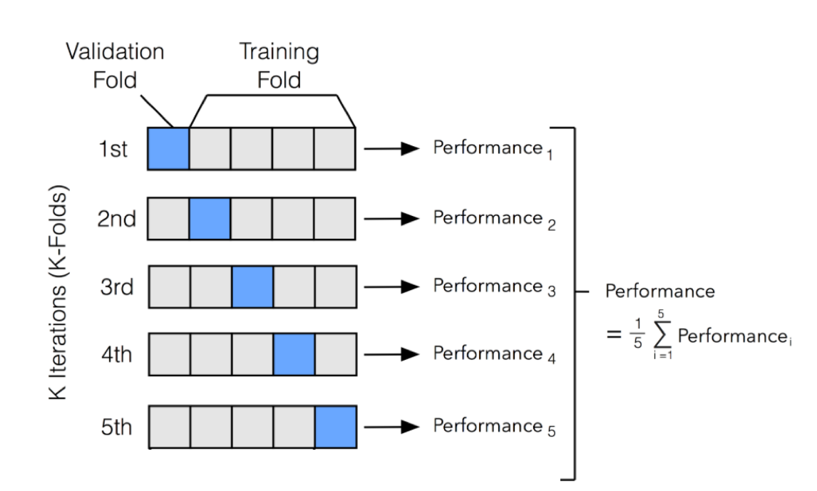
    1. Split the training set into k-subsets: {D1, D2,..Dk} with (almost) equal size. 2. Loop through k iterations. At $i^th$ iteration, select subset Di as validation set and the remaining k-1 subsets as training set. 3. Compute accuracy of each iteration 4. Compute the mean of accuracies obtained in k iterations.
    

  • Leave One out

    1. It is a case of k-fold cross validation with setting K= N, the number of data point in training set.
    2. It hence takes N-1 iterations to evaluate model.
       

  • Stratified Cross validation

    1. It is a case of K-fold cross validation with each setting: each set contains approximately the same percentage of samples of each target class as the complete set.
       __For example:__ In a dataset S= {A1,A2,A3,B1,B2,B3,C1,C2,C3}, which has classes A,B,C. Each class occupies 30% of total dataset.In Stratified 3-fold Cross-validation, S= {K1,K2,K3}. To make each class of data in each fold have the same percentage, we have: K1 ={A1,B1,C1}, K2 ={A2,B2,C2}, K3 ={A3,B3,C3} such that the percentage of each class of sample in each fold is still 30%.
       

  • Note for Cross-Validation

    1. When K is small, the variance in performance of model could be large, since each fold contains more data and hence becomes noisy.
    2. When K is large, eg. in LeaveOneOut, K=N, variance of performance of model would be smaller.
    3. In each fold of training set, we need to start training the initial model again, rather than training the model from the last fold.
    4. Cross validation is to evaluate the performance of the framework of the model, rather than of the parameters of the model.
       

• Bootstrap (Sample-based)

  1. Samples the given training tuples uniformly with replacement d times as training set. The remaining data tuples form the test set (or validation set).
     That is,
     the tuples/samples that have been chosen can still be chosen with equal possibility
  2. Train model with training set
  3. Compute average accuracy of model on both training set and test set
  4. Repeat steps 1~3 k times, then compute average accuracy of all accuracy obtained in k iterations.
     

• Comparison among methods Above

  1. holdout
     Purpose
     Holdout is mainly used to evaluate how well the model performs on the unseen dataset. It evaluates both framework and hyperparameter of the model.
     Different from cross-validation, the holdout data can be any size (usually 20% of the training dataset), while cross-validation requires validation data has the same size as each fold. When the amount of fold is small (like 2) in cross-validation, it could waste the training set.

     
     

     Advantages

     • Less expensive in computation, Easy to compute, compared with cross-validation, since it splits test set randomly

       Disadvantages

     • Estimated accuracy may be unstable (Accuracy is easy to change), since holdout depends on the dataset split methods on training set and test set.

       When to Use

     • When the dataset is very large and hard to compute multiple subset

       
       

  2. Cross-validation
     Advantages

     • The estimated accuracy is much stable than holdout , since it trains model on multiple different train-test set splits. It guarantees to train model with all samples.

       Disadvantages

     • The Cost for computation is expensive when dataset is very large.

     • When value K is smaller, the variance in performance of model will be larger and model is easier to overfit (training with more data samples could be more noisy).

     • When value K is smaller, it could waste the training set. For example, in 2-fold, we use only half of training set to train the model, which is a waste of training data.

       When to Use

     • when dataset is not very large (10000 samples or even more)

     • when you have powerful computational device.

       
       

  3. Bootstrap
     Advantages

     • Performance of model doesn’t depend on the split method on dataset

     • When dataset is small or insufficient, or imbalanced (some classes are more than other significantly), it may reduce overfitting effect by sampling with replacement

     • Less expensive on computation compared with cross validation

       Disadvantages

     • Need to determine what sampling method to use

       When to Use

     • when dataset is small or insufficient (In this case, we may use Over-sampling to repeat some data)

     • when dataset is imbalanced

     • when dataset is pretty large (In this case, we may use down-sampling to select part of data for training)

Comparison of performances among different model

How do we know the performances between models are similar?

• t-Test / Student’s t test Read this paper

Model Selection

• ROC curve: receiver operating charatistic curve (true positive rate -VS- False positive rate)
  we first let model output possibility of each class and then set the threshold to convert possibility to 0, 1 binary classification labels.
  The threshold is usually default as 0.5.
  Based on the binary classification, compute true positive rate TPR/recall (TP/(TP+FN)) and false positive rate/FPR (FP/(FP+TN) = FP/real negative)
  Since threshold is set to 0.5, during training of model, the performance of model will change and hence TPR and FPR will change.
  The changing TPR and FPR leads to the ROC curve

  
  

• AUC: area under curve ( ROC curve)
  Since TPR and FPR range from 0 to 1, hence AUC has range [0, 1]. AUC usually is inside [0.5, 1] because a good model usually can classify sample correctly with 0.5 possibility.

  
  

• Physical Meaning of AUC:
  AUC is the possibility that a random-chosen positive sample is ranked more highly than a randomly-chosen negative sample.
  In other words, AUC is the possibility that a model’s prediction possibility of a random positive sample is more higher than a random negative sample. Then when AUC of a model is larger, it is more likely for the model to predict positive sample as 1 , rather than negative sample as 1.

  
  

• Example: when threshold =0.5
  Case 1

  Sample	A	B	C	D
  Possibility	0.9	0.8	0.51	0.3
  Prediction	1	1	1	0
  Ground Truth	1	1	0	0
  In case 1 we see that possibility that positive sample is ranked higher than negative sample, since all positive sample has possibility greater than negative sample and TPR = 2/2=1 as FPR = 1/2 =0.5 < TPR. Hence in this case, it is a good model.

  Case 2

  Sample	A	B	C	D
  Possibility	0.9	0.3	0.51	0.6
  Prediction	1	0	1	1
  Ground Truth	1	1	0	0

  In case 2, we see that TPR = 1/2 < FPR= 2/2=1 and AUC is small. The possibility that positive sample ranked higher than negative sample is small. The prediction possibilty of positive sample is also small than negative sample in sample B,D. Hence the model performance is not good enough.

Improvement on Accuracy: Ensembling method

• Bagging (bootstrap aggregation)

  • Main Idea:
    Its goal is to reduce variance by using multiple classifiers, like decision tree. It uses boostrap method to sample data and train multiple classifiers and then average the prediction over a collection of classifiers (for continuous value prediction, regression), or return the prediction with maximum votes (for
    classification)
    Random forest is a bagging approach, which bags a set of decision trees together.

    
    

  • Assumptions
    we have training set with size of D and a set of models with size of K

  • Training:

    1. Similar to Bootstrap, at each iteration i, a training set Di of d tuples is sampled with replacement from training set.
    2. A classifier model Mi is learned for each training set Di

  • Prediction:

    1. Each Classifier Mi returns prediction for input X.
    2. Discrete value output: The bagged classifier counts the votes and assigns the class with the most votes to X
    3. Continous value output:
       take the average value of each prediction for a given test sample.

  • Advantages:

    1. Better than a single classifier from the classifier set.
    2. More robust in noisy data and hence smaller variance

  • Disadvantages:
    1.Its training depends on sampling techniques, which could affect the accuracy

    2. The prediction may be not precise, since it uses average value of classifiers’ predictions.
       For example, if valid prediction values are 1,2,or 3, then the average of predictions from different model could lead to a floating point number.

  • Properties of Random Forest

    1. Comparable in accuracy to Adaboost, but more robust to errors and outliers.

    2. Insensitive to the number of attributes selected for consideration at each split, and faster than boosting

       
       

• Boosting

  • Main Idea:
    Its goal is to improve accuracy, let models better fit training set. It uses weighted votes from a collection of classifiers

    
    

  • Training:

    1. Each training sample/tuple is given a weight, eg $w_i$ for the $i^{th}$ tuple. Then we have training set {(X0,y0, w0), … ,(Xi,yi, wi)}
       where $X_i$ and $y_i$ are training sample and target
    2. We have k classifiers {M0, M1,…Mk}. Each classifier is learned from the whole training set iteratively. That is, if we have k classifiers, then we need to iterate the training set at least k times (at $i^{th}$ iteration, we train the $i^{th}$ classifier), so that each classifier can learn the training set.
    3. After classifier $M_i$ is learned on training set, classifier $M_{i+1}$ paies more attention to the training samples that are misclassified by $M_i$
       

  • Prediction:
    The final Model combines the votes of each individual classifier. Either find the prediction with largest sum of weights (Classification), or find the average of all prediction values (Regression)
    The weight of each classifier’s vote is a function of its accuracy

    
    

  • Advantages

    1. Boosting can be extended to numeric prediction
    2. Better fit the training set since it adjusts the weights of training set and gives more attention to the misclassified sample.
       

  • Disadvantages

    1. Easy to overfit. Need Additional techniques to avoid overfitting. (I will discuss the methods dealing with Overfitting ).
       

  • Questions:

    1. How to pay more attention to misclassified samples? give Higher weights? But How to compute weights?
       Answer: This depends on the actual boosting algorithm, like GradientBoosting, AdaBoosting
       

  • AdaBoosting

    1. Assumption:
       Assume we have training set with size of D and a set of classifier models with size of T

    2. __Error of model $M_i$__

       Error($M_i$) = $\sum_i^D (w_i \times err(X_i))$

       if using normalized weight (weight in range [0,1]), then
       Error($M_i$) = $\frac{\sum_i^D (w_i \times err(X_i))}{(\sum_j^D w_j)} $

       
       

       Note:
       In classification, $err(X_i)= 1(C_i(X_i) !=Y_i)$, $C_i(X_I)$ means the prediction of model $M_i$ on sample $X_i$. If the prediction is correction $error(X_i) =0$, otherwise 1.

       
       

    3. Weight of model $M_i$’s voting: $\alpha_i$
       $\alpha_i = log\frac{1-error(M_i)}{error(M_i)} + log(K-1)$.

       Note:
       K = the number of classes in dataset. When K=1, log(K-1) term can be ignored

       
       

    4. Update of weight
       $w_i = w_i \cdot exp(\alpha_i \cdot 1(M_j(X_i) != Y_i))$

       
       

       The weight $w_i$ of the $i^{th}$ training tuple $X_i$ is updated by timing exponential value of weight of model only when this model $M_j$ misclassifies the $X_i$ ( That is $M_j(X_i) !=Y_i$ and hence $1(M_j(X_i) !=Y_i) =1 $).

       
       

    5. Prediction
       $C(X_i) = argmax_{k} \sum_{j=1}^T \alpha_{m}\cdot 1(M_j(X_i)== Y_i)$
       where $1(M_j(X_i)== Y_i)$ is equal to 1 if prediction is correct, otherwise, 0.
       The prediction of the whole model has the largest sum of weight of models, NOT the weight of training tuple!

       
       

    6. More detail for AdaBoosting, Read this paper

       
       

• Stacking

  • Main Idea:
    It combines and trains a set of heterogeneous classifiers in parallel.
    It consists of 2-level models:
    level-0: base model
    Models fit on the training data and whose predictions are compiled.
    level-1: Meta-Model
    It learns how to best combine the predictions of the base models.

    
    

  • Training:

    1. split the training data into K-folds
    2. one of base models is fitted on the K-1 parts and predictions are made for Kth part.
    3. Repeat step 2 for each fold
    4. Fit the base model on the whole train data set to calculate its performance on the test set.
    5. repeat step 2~4 for each base model
    6. Predictions from the train set are used as features for the second level model.
       

  • Classification:
    Second level model is used to make a prediction on the test set.

    
    

  • Advantage:

    1. It harness the capabilities of a range of well-performing models on a classification or regression task and make predictions that have better performance than any single model in the ensemble.
       

  • Disadvantage:

    1. It could be computational expensive since it uses k-fold method and use multiple level models.
       

• Comparison among Ensembling, boosting and bagging

  1. Goal of bagging is to reduce variance and noise while boosting is to improve accuracy using weighted models. Stacking is to improve accuracy of model using hetergenerous models.
  2. Adaboost let classifiers pay more attention to the misclassified samples, but if those misclassified samples are outlier or noisy data, it will affect a lot and lead to larger variance.
     However, bagging and ensemble uses averaging and voting methods and each classifier has equal weight, which is less sensitive to the noise data and outlier.

Reference

[1] https://blog.csdn.net/weixin_37352167/article/details/85028835
[2] https://machinelearningmastery.com/stacking-ensemble-machine-learning-with-python/
[3] https://en.wikipedia.org/wiki/Student%27s_t-test
[4] https://media.springernature.com/lw685/springer-static/image/art%3A10.1038%2Fnmeth.3945/MediaObjects/41592_2016_Article_BFnmeth3945_Fig1_HTML.jpg