Data Structure 2 -sorting

Bubble sort (冒泡排序法)

Main idea

Bubble sort compares the array elements $(n-1) + (n-2)+…+1 = \frac{n(n-1)}{2}$ times. At $k^{th}$ iteration, iterate (n-k) elements and swap two elements if previous one is larger than the next one in ascending sorting.
It guarantees that in each iteration, there must be at least one element sorted into the correct positions
Example:
in an array [5 1 4 2 8] with length = 5
Begin:
$1^{st}$ iteration: iteration starts from arr[0] to arr[4] and swap two element if arr[i] > arr[i+1].
[5 1 4 2 8] $\to$ [1 5 4 2 8] $\to$ [1 4 5 2 8] $\to$ [1 4 2 5 8] $\to$ [1 4 2 5 8]

$2^{nd}$ iteration: iteration starts from arr[0] to arr[3] and swap two element if arr[i] > arr[i+1]. Process is similar to the first iteration.
The result is [1 4 2 5 8] $\to$ [1 2 4 5 8]

$3^{rd}$ iteration: iteration starts from arr[0] to arr[2].
$4^{rd}$ iteration: iteration starts from arr[0] to arr[1].
End

Process

1. Pesudo Code

   Loop through n-1 iteration:
       at the k^th iteration, loop through arr[0] to arr[n-1 - k] element:
           if arr[i]> arr[i+1]
               swap arr[i], arr[i+1]

2. Python Code

   def bubble_sort(array):
       n = len(array)
       for i in range(n-1):
           for j in range(n-1-i):
           if array[j] > array[j+1]:
               array[j], array[j+1] = array[j+1], array[j]
       return array

   Complexity

• Memory Complexity: O(1), since there is no memory used in algorithm
• Time Complexity: O(n^2), since there are two inner loops in function and need $\frac{n(n-1)}{2}$ comparison.

Selection Sort (选择排序法)

Main Idea

Selection sort is to find the maximum value of current array and put it to the end of array and then exclude this sorted element to get the sub-array and repeat these two steps to sort the array. If find minimum value, need to put it to the beginning.

Process

1. Pesudo Code

   Loop through n-1 iterations 
       at k^th iteration
       find max of array[0:n-1-k]
       put max into array[n-1-k]

2. Python Code

   def selection_sort(array):
       n = len(array)
       for i in range(n):
           max_v = 0
           for j in range(n-i):
               if array[max_v] < array[j]:
                   max_v = j
           array[n-i-1] , array[max_v] =array[max_v], array[n-i-1]
       return array

   Complexity

• Memory Complexity: O(1) since in this code, we don’t use additional memory
• Time Complexity:: O(n^2), since selection sort use two loops to sort. One inner loop is used to find max value and the other loop is to sort the max values.

Insertion sort (插入排序法)

Main Idea

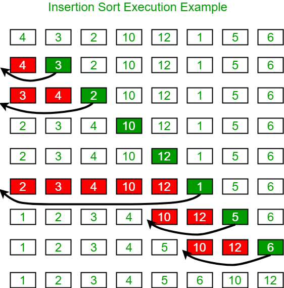
Main idea of Insertion Sort is to compare the current element with elements before this element and then insert this element to the correct position by moving some elements backward.

1. Start from arr[1], i=1. Iterate elements arr[i] with index i from 1 to N-1
2. For each element arr[i], compare arr[i] with the element arr[k] right before arr[i]. If we found element arr[k] > arr[i], swap arr[i] and arr[k].
3. Repeat Step 2 until the element arr[k] before arr[i] is less than or equal to arr[i]
   Example:
   Given an array arr = [4,3,2,10,12,1,5,6] with array length N= 8, initial index =0, we want to sort it in ascending order.
   iteration 1: [4,3,2,10,12,1,5,6] $\to$ [3,4,2,10,12,1,5,6]
   iteration 2: [3,4,2,10,12,1,5,6] $\to$ [3,2,4,10,12,1,5,6] $\to$ [2,3,4,10,12,1,5,6]
   …

Process

1. Pseudo code

   Let i = 1
   Loop until i ==N-1
       j= i-1
       // swap arr[i] and arr[j] if arr[j]>arr[i]
       while arr[i]< arr[j] and j>0:
           swap(arr[i], arr[j])
           j--
       i++

2. Python Code

   def insertion_sort(array):
       for i in range(1,len(array)):
           j = i-1
           while j>=0  and array[j] >array[j+1]:
               array[j],array[j+1] = array[j+1], array[j]
               j -= 1
       return array

   Complexity

3. Memory Complexity: O(1)
4. Speed Complexity:
   • worst case: O(n^2)

Extension

1. Binary Search + Insertion sort. Reference

Quick sort (快速排序法)

Main Idea

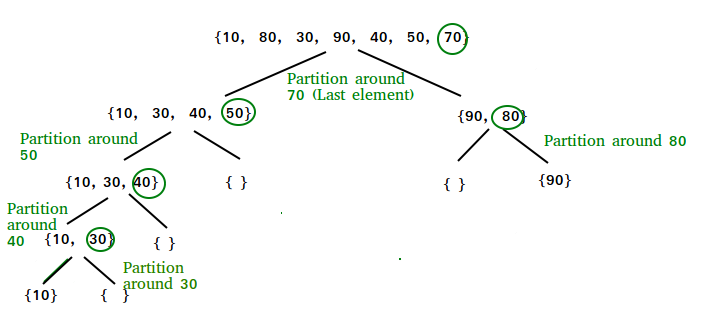
In quick sort, the main idea is that

1. we first choose a pivot/key element used for comparison. Usually we choose the last element in the partition/array as the pivot (we can also choose middle element or the first element as well)

2. Move the elements smaller than pivot to the left to form a subarray/partition P1 containing all elements smaller than pivot.

3. Move the elements larger than pivot to the right to form a subarraysubarray/partition P2 containing all elements larger than pivot

4. Move pivot to the position between P1 and P2 such that elements ahead pivot are smaller than pivot, elements after pivot are after than pivot
   Note: This structure is actually as same as binary search tree, in which elements on the left side of the parent node is smaller than parent as elements on the right side of the parent node is greater than parent

5. Repeat steps 1~4 for each partition recursively until subarray can not be partitioned (only one element)

Process

1. In Partition step

   • set the last element arr[len(arr)-1] to be pivot

   • set pointer pointing to values smaller than pivot: left_pt =0 and pointer pointing to values greater than pivot: right_pt = len(arr)-2

   • Loop until reaching terminal state: left_pt> right_pt

   • left_pt++ until it finds arr[left_pt]>pivot

   • right_pt– until it finds arr[right_pt]< pivot

   • swap arr[left_pt] and arr[right_pt]

   • after reaching terminal, swap pivot and arr[left_pt] such that pivot is at the correct position.

   • Pseudo Code

     partition(array, low, high):
         // check if input range is valid 
         if begin-end < 1:   return end
         
         pivot = array[high]
         left_pt = low
         right_pt = high-1
         //move left_pt to right, right_pt to left until  left_pt>right_pt
         //when left_pt>right_pt, we know array[left_pt] >= array[right_pt]
         //then we need to swap pivot with either array[left_pt] or array[right_pt]  to set the boundary
     
         Loop if left_pt<= right_pt:
             Loop if left_pt< len(array) and array[left_pt] <= pivot:
                 left_pt++
             Loop if right_pt> 0 and array[right_pt]>= pivot:
                 right_pt--
             
             if left_pt< right_pt:
                 swap array[left_pt] and array[right_pt]
         if array[left_pt] > pivot
             swap array[left_pt], pivot
         return left_pt

     Note:

   • array may have multiple values as same as pivot. In order to iterate each element in position 0~n-1, need to use <= pivot, and >= pivot to avoid trapping at some positions that doesn’t satisfy terminal condition
     eg.

     arr[left_pt]	a[1]	arr[right_pt]	arr[pivot]
     2	1	2	2

     In this case, if we use “< pivot” and “>pivot” rather than “>=”,”<=”, then left_pt and right_pt won’t check “1” in the array.

   • __Need to compare array[left_pt] and pivot__, since when the input array has only 2 element, then left_pt = right_pt, it directly skips the loop and swap data without comparing the values, this could be wrong.

     
     

2. Pseudo Code

   QuickSort( array):
       return quicksort(array, 0, len(array)-1)

   quicksort(array, begin,end)
       //Check if array is empty or length >1
       if end-begin<1: return array
       
       // find the correct position of pivot
       mid = Partition(array, 0, len(array)-1)
       // sort the subarray with elements smaller than pivot
       array = quicksort(array, 0, mid-1)
       // sort the subarray with elements greater than pivot
       array =  quicksort(array, mid+1,len(array)-1)
       return array

3. Python Code

   class Solution(object):
       def quickSort(self, array):
           """
           input: int[] array
           return: int[]
           """
           # write your solution here
           if array == None or len(array)==0:
           return array
           begin = 0
           end = len(array)-1
           return self.quick_sort(array, begin,end)
   
       def quick_sort(self, array, begin, end):
           # Check base case
           if begin >=end:
               return array
           #pre-order operation
           
           # partition
           l_begin, l_end, r_begin, r_end = self.partition(array, begin, end)
           # recursively go to left and right sub-array
           array = self.quick_sort(array, l_begin, l_end)
           array = self.quick_sort(array, r_begin, r_end)
           return array
       
       def partition(self, array, begin, end):
           # check base case
           if begin >= end:
               return begin, begin, begin,begin
           # choose pivot
           import random
           # randomly choose a pivot in array
           # then move the pivot to the end of the array, pivot=end
           pivot = random.randint(begin, end)
           array[pivot], array[end] =  array[end], array[pivot]
           pivot = end
           stored_index = begin
           for i in range(begin, end+1):
               if array[i] < array[pivot]:
               array[i], array[stored_index] = array[stored_index], array[i]
               stored_index += 1
           array[pivot] , array[stored_index] = array[stored_index], array[pivot] 
           l_begin = begin
           l_end = stored_index-1
           r_begin = stored_index +1 
           r_end = end
           return  l_begin, l_end, r_begin, r_end

Complexity

• Memory Complexity: O(1) if we don’t consider the memory in stack. Otherwise, O(logn)

• Time Complexity:

  • best case/average case；O(nlogn)
  • worst case: O(n^2), since it is possible that every time we select the pivot of sub-array is the largest element of this sub-array, which lead to the case that the recursion tree becomes linked list.
    When the Recursion tree becomes linked list, time complexity becomes O(nh) = O(nn) rather than O(nh) = O(nlogn), where h is the height of tree.

  To solve this problem, we can use random selection method to select the pivot, rather than always pick the last element as pivot

  Note

• when it always picks the greatest/ smallest value as pivot or the array is already sorted, it comes to the worst case O(n^2) since the recursion tree becomes a list-like data structure with depth of recursion tree = O(n) and take O(n) to iterate every node and O(n) to sort at each node. Then it comes to O(n*n) time complexity

• Quick Sort use Pre-Order, Top-down, in-place operation to first partition array and then do recursion

• Merge Sort use Post-Order, Bottom-up, not in-place method to return array and then merge returned array

Merge sort （归并排序）

Main Idea：

Merge sort is one of the divide and conquer algorithm like quicksort. Its main ideas is that

1. Find the middle of the array
2. Divide the array into two sub-array based on middle
3. Repeat step 1~2 recursively until only 1 element in the array
4. Merge left array and right array and return merged array recusively
5. Example:
   In the array below, we recurively divide the array into left sub-array 2 and right sub-array 12, then sort the left array first by dividing it until step 4,5. We then merge two elements in step 6. After that, we go back to step 2 to sort the right sub-array. We do the same thing for the whole array.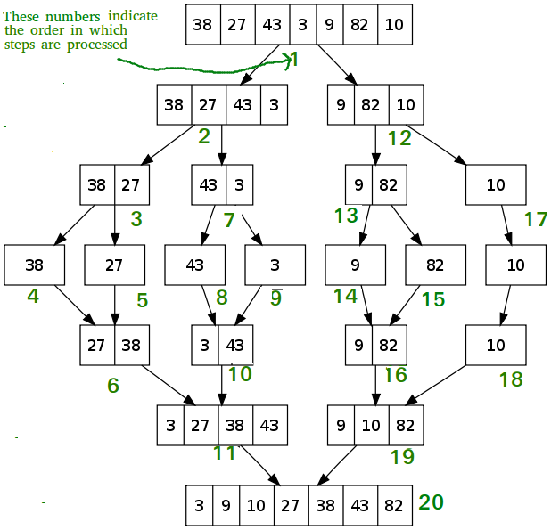

Process

1. Pesudo Code

   MergeSort( array)
       check if array is valid array, if not ,return
       compute left , right boundary
       merge_subarray(array, left, right)
   
   merge_subarray(array, lef, right):
       check if left < right. If not, return array[left]
   
       compute middle = (left+right)//2
       // sort left array
       left_array = merge_subarray(array, left, middle)
       // sort right array
       right_array = merge_subarray(array, middle+1, right)
       // merge and sort left and right arrays
       sorted_array = merge(left_array, right_array)
   
       return sorted_array
   merge(left_array, right_array):
       use linear method to merge the left array and right array.
       // Note that since left_array and right array have 
       //been sorted, merging two sorted array actually 
       //lead to linear time complexity O(n) only
       create new array A
       left_index = 0
       right_index = 0
       while left_index >0 and right_index>0:
           add the min(left_array[left_index], right_array[right_index])
           index += 1
       Add the remaining elements in array to A
       return A

2. Python code

   class Solution(object):
       def merge_sort(self, array, left, right):
           if len(array)<2 or left>=right:
           return [array[left]]
   
           middle = left+ (right-left)//2
           left_array = self.merge_sort(array, left, middle)
           right_array = self.merge_sort(array, middle+1, right)
           sorted_array = self.merge(left_array, right_array)
           return sorted_array
       
       def merge(self, left_array, right_array):
           if left_array == None or len(left_array) <1:
           return right_array
           elif right_array == None or len(right_array) <1:
           return left_array
           
           l_index = 0
           r_index = 0
           merged_array = []
           while l_index < len(left_array) and r_index<len(right_array):
           if left_array[l_index] <  right_array[r_index]:
               merged_array.append(left_array[l_index])
               l_index += 1
           else:
               merged_array.append(right_array[r_index])
               r_index += 1
           if l_index < len(left_array):
           merged_array.extend(left_array[l_index:])
           elif r_index < len(right_array):
           merged_array.extend(right_array[r_index:])
           return merged_array
   
       def mergeSort(self, array):
           """
           input: int[] array
           return: int[]
           """
           # write your solution here
           if array == None or len(array) <2:
           return array
           
           return self.merge_sort(array, 0, len(array)-1)

   Complexity

• Memory Complexity: if consider the memory used in stack during recursion, it is O(logn)
• Time Complexity: O(nlogn). In each layer of recursion tree, it takes O(n) to merge and sort two sub-arrays at a level of the tree. Since merge sort uses division method, that is, Assume that are n elements to sort and take k steps (depth of the recursion tree) to sort. There are $2^0+2^1+…+2^k = n$ elements. When only consider the largest term, we have $2^k = n$, and $k = O(log_2n) or O(logn)$. Since each level of recursion tree take O(n) to sort array, then have $O(nlogn)$

Compared with quick sort

1. Both merge sort and quick sort use divide and conquer method (分治算法) to divide array and then solve each subset recursively. Hence both of them involve logn time complexity
2. As for memory complexity, merge sort has O(nlogn) while quicksort has memory complexity O(logn). Quicksort is better than mergesort
3. As for time complexity, merge sort has average/worst case time complexity: O(nlogn) while quick sort has O(nlogn) in average case and O(n^2) in worst case. Quick sort is less stable than merge sort.
4. Quicksort and merge sort are much more useful than linear sorting(insertion, bubble, selection) due to its O(nlogn) time complexity without increasing memory complexity

Notes:

1. Usually, Recursion method is less optimal than iteration method (using while loop), since recursion method requires stack memory to store and return solved subset back to last sub-problem. Hence memory complexity of recursion is usually O(n) unless there are no memory used in recursion function and reduce n to 1
2. Recursion method is easy to implement, but usually costs more memory.
3. Selection sort can be viewed as a version of bubble sort with more explicit physic meaning, since it explicitly finds the min/max value and put them to the beginning/end of subarray.
4. Insertion sort compares current element with previous elements while bubble/selection sort compare current element with the next elements
5. In-place algorithm: an algorithm which transforms input using no auxiliary data structure. However a small amount of extra storage space is allowed for auxiliary variables. The input is usually overwritten by the output as the algorithm executes.

Source code

For C++ source code, Please read my github repository here

Reference

[1] https://www.geeksforgeeks.org/bubble-sort/
[2] https://www.geeksforgeeks.org/insertion-sort/?ref=lbp
[3] https://www.geeksforgeeks.org/quick-sort/?ref=lbp