ML Model - Regression models

Introduction

This article is to first introduce types of machine learning models and summarize properties of seven regression models: Linear Regression and Logistic Regression, Lasso Regression, Ridge Regression, Elastic Net Regression and Stepwise regression.

Type of machine learning model

Parametric/ non-parametric models

In general, Machine Learning model can be classified into two types of models based on the critic that if model uses parameters to estimate model or not.
In this case, machine learning model can be divided into two types: parametric model and non-parametric model.
The following are some useful machine models:

• parametric:
  • Linear regression, Logistic regression
  • Neural Network
• non-parametric:
  • K-Nearest neighbor (K-NN)
  • K-Mean Clustering
  • Decision Tree
  • Random Forest
  • Naive Bayesian
  • etc…
    Note that the “parametric” here is the parameters the model use to estimate the function, distribution. The parameters that control the complexity, performance of model are excluded. For example, K-Mean clustering and K-NN requires us to choose a k value to do clustering/ classification tasks. This k value is not the parameter we consider here.
    

linear/non-linear model

1. Linear model
   The linear model is the model that can be expressed by the formula
   $y’ = w_0 + w_1x_1 +….+w_nx_n = w_0+ \sum_{i}^nw_ix_i$
   where x is the data point from dataset, $w_i$ is the parameters used to adjust the model and $w_0$ is the bias term. $y’$ is the prediction from the estimator.
   This formula is linear since it just involves first order terms and linear combination.
   Note that the real label is
   $y = \epsilon + w_0+ \sum_{i}^nw_ix_i$
   where $\epsilon$ is the irreducible error between prediction $y’$ and true label $y$. In the following discussion, I discuss $y’$ prediction from model rather than label $y$.

2. Non-linear model
   Non-linear model in other word is the model that can not be expressed by the linear formula above. If there are second order term like $x^2, x^3, x_1x_2$, it is non-linear model as well
   Hence we can easly know that models like Naive Bayesian, K-NN, K-mean clustering, logistic regression, etc are non-linear models

   
   

Linear Regression

The formula of Linear Regression is
$$y’ = w_0 + w_1x_1 +….+w_nx_n $$
where $w_0$ is a constant and $y’$ is the prediction from model. To simplify it, we have:

$$y’ = \sum_{i=1}^nw_ix_i + w_0$$
Obviously, the linear regression model is a linear model.

Optimize Model

1. Maximum Likelihood Estimation (MLE)
   Assume the data distribution is normal distribution, then
   the likelihood function used to estimate the real data distribution is:

   $$P(y=y_i|x) = \frac{1}{\sigma\sqrt{2\pi}} e^{-\frac{(y_i-f(x))^2}{2\sigma}}$$

   where f(x) is the linear regression estimator, estimating the mean of normal distribution $\mu$. Then the weight solution of the regression model is

   $$W = argmax_w P(Y|X)$$

2. Loss Function to minimize
   The loss function used to update the parameter in Linear regression is mean square error (MSE)

   $$ MSE = \frac{1}{N}\sum_i^N{ (y_i - y’_i)^2 }$$

   or sum square error (SSE)

   $$ SSE = \sum_i^N{ (y_i - y’_i)^2 }$$

   where $y_i$ is the $i^{th}$ label and $y’_i$ is the $i^{th}$ prediction from model

   Properties of MSE/SSE:
   SSE / MSE error actually assumes that the distribution of data is Normal distribution and the Linear regression model is actually estimating the mean of Normal distribution with a fixed variance $\sigma$. The negative log likelihood of normal distribution is as follow:

   $$ -log(\Pi_i^nP(y=y_i|x_i)) \
   \propto -log(e^{\sum_i^n\frac{-(y_i-f(x_i)^2)}{2\sigma}}) \
   \propto \sum_i^n(y_i-f(x_i))^2
   $$
   where $y_i$ is the $i^{th}$ label and $x_i$ is the $i^{th}$ feature vector.
   It is easy to see that maximize the likelihood function is equivalent to minimize the negative log likelihood function or the SSE /MSE.
   Hence to minimize the MSE error is actually estimating the normal distribution function $P(Y|X)$.

   
   

Properties

1. Linear regression is an unbias model, which is sensitive to outliers.For example, In the following linear regression

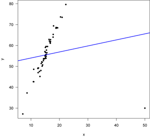
There is an outlier at x= 50, y= 30.
During update with gradient descent w = w - 2x(y - wx). The outlier value changes the weight a lot and shift the line away from the $y=4x$. This is because in the update of parameter $w$, each data point is given equal weight to change the parameter $w$.
Hence linear regression is sensitive to outliers.

2. The output/prediction from linear regression is to estimate the expected value/ mean of normal distribution
   

Logistic Regression

Logistic regression is an non-linear model as it can not be expressed into the linear form.
The formula of Logistic Regression model:

$$ P(y=y_i|x) = p_i = \frac{1}{1+e^{-wx}} $$

Optimize Model

1. Maximum Likelihood Estimation (MLE):
   we want to maximize the log likelihood function (The distribution estimated by the model) to get close to the real distribution function.

   In binary classification problem, we assume the data distribution is Bernoulli distribution, $ P(y=y_i|x) = p^{y_i}(1-p)^{1-y_i}$， since this distribution considers the possibility of P(y=0|x) and P(y=1|x).
   Then the log likelihood function / log Bernoulli distribution is following:

   $$ logP(y_1,y_2,..y_n| x_1, x_2..x_n) =log(P(y_1|x_1)P(y_2|x_2)..P(y_n|x_n))$$

   $$ =\sum_i^n log(p_i^{y_i}(1-p_i)^{1-y_i})= \sum_i^n[y_ilog(p_i)+(1-y_i)log(1-p_i)]$$

   Since we only care the effect of weight vector and data X to the likelihood function, it can be re-written as

   $$ \sum_i^n[y_ilog(h_w(x_i))+(1-y_i)log(1-h_w(x_i))]$$

   where $x_i, y_i$ are feature vector and binary label, $h_w(x_i) = p_i$ is the logistic regression, estimating the possiibility that if $x_i$ belongs to class 0 or class 1.
   The log function here is used to simplify the likelihood function and convert the multiplication into summation. This gives us easier way to analyze it. Maximizing the log likelihood is equivalent to maximize the original likelihood function.

   Notice that when $p_i$ predicted by the model is as same as its label $y_i$, then $p_i^{y_i}(1-p_i)^{1-y_i}$=1, the likelihood function is maximized.
   The optimal solution of weight matrix in logistic regression is

   $$W = argmax_W (\sum_i^n(y_ilog(h_w(x_i))+(1-y_i)log(1-h_w(x_i))))
   $$

   
   

2. Binary Cross-Entropy
   When we add the negative sign to the log likelihood function, we can get

   $$ - \sum_i^n log(p_i^{y_i}(1-p_i)^{1-y_i})= -\sum_i^n(y_ilog(p_i)+(1-y_i)log(1-p_i))
   $$

   This form is also called binary cross-entropy. To maximize the likelihood function to real distribution of data, is actually equivalent to minimize the binary cross entropy. Cross entropy is to measure the uncertainty between $y_i$ and $p_i$, $1-y_i$ and $1-p_i$. Higher the entropy is, less similar they are. So binary cross entropy assume the data is in Bernoulli distribution

   The goal to train the logisitic regression using binary cross-entropy is to let $h_w(x_i)$ get as close to $y_i$ as possible.

Properties

1. Logistic function actually projects the range of linear regression into range of [0,1]. Y-axis in logistic regression= possibility that input x belongs to one class, while the linear regression output range is ($-\infty, +\infty$).

2. Logisitic regression is an bias model, since it considers the feature values X close to 0 are different and hence the gradient close to x=0 is large. However, when x is far away from x=0, such as $+\infty, -\infty $, the gradient of logistic function is close to 0 and it “considers” there is no much difference between two features x1 and x2 when both x1 and x2 $\to \infty$.

3. Logistic Regression has vanishing gradient problem.
   Since the gradient of logistic regression is :

   $$(\frac{1}{1+e^{-wx}})’ =\frac{ e^{-wx}}{(1+e^{-wx})^2} = (\frac{1}{1+e^{-wx}})(1-\frac{1}{1+e^{-wx}})$$

   when it predicts some sample X as a value very close to 0 or 1, the gradient will be very close to 0 and the weight is hard to update any more. The gradient is actually vanishing in this case. When it think a sample X is class y, then it won’t be willing to change its mind. This is a reason why it is “biased model” as well

4. Logistic Regression is widely used for binary classification problem, it can be regarded as a two-classes version of softmax function.

5. Using Maximum Likelihood estimation requires large data sample size in order to estimate the real distribution.

6. Assumption in Logistic Regression is that the logarithem value of the ratio of possibility of class =1 to possibility of class =0 is linear, which can be estimated by linear regression.
   Proof:
   $$
   log(\frac{P(Y=1|X)}{P(Y=0|X)}) = log(\frac{P(Y=1|X)}{1- P(Y=1|X)})=wx \
   $$

$$
(1- P(Y=1|X))*e^{wx} = P(Y=1|X)
$$

$$
P(Y=1|X) = \frac{e^{wx}}{1+e^{wx}} = \frac{1}{1+e^{-wx}}
$$

7. Logistic Regression is to find a linear separation boundary /a line that separate the data in sample space for classification problem. Since in logistic regression $\frac{1}{1+e^{-wx}}$, when $-wx>0$, $h_w(x)>0.5$ and it predicts class 1, otherwise, class 0. The line $-wx=0$ in 2-D space shown in the left figure below is actually the decision boundary. The data x with $-wx>0$ is above the line and is classified as class1.

Polynomial Regression

$$
y’ = w_0 + w_1x_1 + w_2x_2^2 +w_3x_3^3+…w_nx_n^n
$$
where y’, $w_i$, $x_i$ are all scalar values in this case and y’ is the predicted value from model. Different from linear regression, polynomial regression involves higher order terms.

Optimize Model

Sum square error
$$ SSE = \sum_i^N{ (y_i - y’_i)^2
}$$
It is as same as the linear regression

Properties

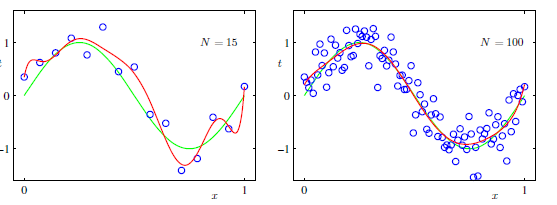
1. It is very easy for Polynomial regression to over-fitting as the order increase. It is an biased model as well.
2. It predicts the expected value of Y, which is as same as linear regression
3. To implement polynomial regression, we can first construct polynomial features, like $x_1^2, x_1x_2, x_2^2$, etc. Then apply linear regression to polynomial features
   

Lasso regression

The prediction model of lasso regression is still linear regression:
$$y’=\sum_{i=1}^nw_ix_i +w_0
$$

Optimize Model

1. Loss function to minimize in Lasso regression:

   $$min \sum_i^n(y_i - wx_i -w_0)^2 + \lambda||w||_{1}$$

   where $y_i$ is a scalar value, a label, $x_i$ is a feacture column vector, $w$ is the weight vector. $\sum_i^n(y_i - wx_i)^2$ is the least square error (or called L2 norm distance between y and x).
   Note that mean square error is scaled version of sum square error. Minimize the sum square error is equivalent to minimize the mean square error, so this term is as same as loss function in Linear regression

   The second term in the loss function is the L1- regularization term used to reduce overfitting effect, in which $||w||_1 = \sum_i^n|w_i|$ is the L1 norm format.

2. Principle of L1-Regularization term

   $$min \sum_i^n(y_i - wx_i -w_0)^2 + \lambda||w||_{1}
   $$

   is equivalent to optimize the problem:

   $$min \sum_i^n(y_i - wx_i -w_0)^2 \
   \text{ subject to } ||w||_1 \leq C
   $$

   where C is a constant.
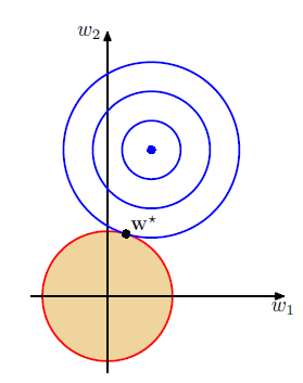
   Assume there are two variables in feature vector $x_i$ and only two weight variables, then to visualize it in 2-D space, we have: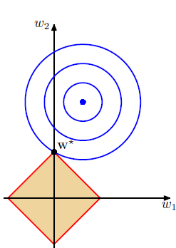

   

   The x, y axis represent the weight variables. The blue point is the optimal point of the minimum least square error term. The orange region describes the constraints $||w||_1 \leq C$, hence the intercepts on x, y axis are equal to $C$.
   The main idea of L1 regularization term is that when the weight vector satisfies the constraint, then the weight vector must be inside the orange region. We need to find the point with the smallest distance to blue point inside this region. When C is small enough such that weight vector can not reach the optimal point, then the model can reduce over-fitting effect.

   By using lagrange multiplier, the constraint problem can be converted to:

   $$min \sum_i^n(y_i - wx_i-w_0)^2 + \lambda (||w||_{1}-C)
   $$

   where $\lambda$ is the lagrange multiplier coefficient used to weigh the regularization term and $\lambda$ is adjusted by user manually. Larger $\lambda$ is, more regularization term affect. We can see that during minimization process, $C$ and $\lambda$ are actually constants, so we can ignore this term and get:

   $$min \sum_i^n(y_i - wx_i)^2 + \lambda||w||_{1}
   $$

Properties

1. It involves L1 regularization term to limit the range of weights and reduce over-fitting effect
2. Lasso regularization can be used to do feature selection
   Since in the figure above, we can see when the optimal solution to this constraint problem is at one of the angles of the square, some weight parameters are driven to be 0 and this leads to a sparse model. That is, the model filters out some features in $x_i$. As $\lambda$ increases, more weights are driven to 0 and more features are not selected.
3. We can not decide which features should be excluded in Lasso regression, since we don’t know which parameters become 0.
4. Feature selection with lasso regression is not stable. Since during training the model, some weights may be very close to 0, but not equal to 0. That is, the features that are expected to be filtered out are actually not filtered out and still affect the model performance.
   In addition, different initialization of weights may lead to different feature selection.
   

Ridge Regression

The prediction model of Ridge regression is linear regression as well:

$$y = \sum_{i=1}^nw_ix_i +w_0
$$

But the loss function is different. Read the following.

Optimize Model

1. Loss function to minimize in Ridge regression:
   $$min \sum_i^n(y_i - wx_i -w_0)^2+ \lambda||w||_{2}^2$$

   Ridge regression is similar to Lasso regression, except that the regularization term here use L2 norm distance. Then the constraint region in 2-D space becomes a circle, shown in below.

   

   Since the constraint region becomes a circle, it is almost impossible to drive some weights to be zeros unless the blue point (optimal point of least square error) is on the axis. Hence, Ridge regression can not be used for feature selection.

Properties

1. Ridge regression can not be used for feature selection
2. Ridge regression can be used to reduce multi-collinearity effect of features and soothe the over-fitting effect.
   multi-collinearity means that some features have a linear correlated relationship. For example, one feature value increases, another feature value may increase or decrease linearly. If model focuses on the similar features, it may become over-fitting on such feature.

The reason is that in the circle region, assume features $x_1$ and $x_2$ are collinear, if $w_1$ increases and the model weigh more on feature $x_1$, then $w_2$ will decrease and model weighs less on feature $x_2$. In this case, model could avoid focusing on learning similar features heavily and reduce the multi-collinearity effect.
3. Reduce the variance in model error and reduce over-fitting effect

4. Ridge regression is more stable than Lasso regression for avoiding over-fitting
   

Elastic Net Regression

The prediction model of Ridge regression is linear regression as well:

$$y’ = \sum_{i=1}^nw_ix_i +w_0$$

Optimize Model

1. Loss function to minimize
   $$min \sum_i^n(y_i - wx_i- w_0)^2 + \lambda_1||w||_{1} + \lambda_2 ||w||_{2}
   $$

where $y_i$ is the label, $w$ is the weight vector and $w_0$ is the scalar bias. $x_i$ is the feature vector.
Elastic net regression combines L1, L2 regularization terms together. Hence it can be regarded as the combination of weighed Ridge regression and weighed Lasso regression.

Properties

1. Combine the advantages of Lasso regression and Ridge regression.
   

Stepwise Regression

In statistics, stepwise regression is a method of fitting regression models in which the choice of predictive variables is carried out by an automatic procedure.
Since there are multiple variable / features in feature vectors, we want to select the most important features to construct our regression model. Different combinations of variables lead to different regression model. Stepwise regression is to select the different feature variables and fit different models and then get the best one with least Residual sum square error

Stepwise regression approaches

Assume there are p features in dataset to pick. There are several types of approaches in stepwise regression for variable selection.

1. Forward Stepwise Regression /selection

   • Begin with the null model { a model that contains an intercept but no predictors.
   • Fit p simple linear regressions and add to the null model the predictor that results in the lowest RSS.
   • Add to that model the predictor that results in the lowest RSS among all two-predictor models.
   • Continue until some stopping rule is satisfied, for example when all remaining variables have a p-value above some threshold. P-value is to measure how significantly different two models are using statistic technique
   • There are p(p+1)/2 models to evaluate

2. Backward Stepwise Regression (Backward elimination)

   • Start with all predictors in the model.
   • Remove the predictor with the largest p-value { that is, the predictor that is the least statistically significant.
   • The new (p -1 )-predictor model is fit, and the predictor with the largest p-value is removed.
   • Continue until a stopping rule is reached.
   • There are p(p+1)/2 models to evaluate

3. Bidirectional Stepwise Regression

   • combine two methods above to see which predictor should be included or excluded from model

Subset Selection

Subset selection is another variable selection method, in addition to stepwise regression

• Assume there are p features in dataset to pick
• fit all models for all subset
• pick the best model with smallest residual sum square error
• There are $2^p$ models to evaluate
  

Summary

This article summarizes the seven regression methods and their properties.
Key things to note:

• Linear regression is to estimate the mean of normal distribution
• MSE assumes data is in normal distribution
• Logistic regression is an biased model to estimate the possibility that input x belongs to a class. Logistic regression assume data is in Bernoulli distribution.
• Binary cross entropy assumes data distribution is Bernoulli distribution
• Lasso Regression (L1 regularization) is good to do feature selection, but could be unstable. It can also reduce the over-fitting effect
• Ridge Regression can not be used for feature selection, but is good to reduce multi-collinearity effect and avoid overfitting
• Elastic Net Regression combines Lasso and Ridge regression
• Stepwise Regression and Subset selection are used to combine and select feature variables to find the estimators with the least SSE error.

Reference

[1] Stepwise Regression

[2] https://www.analyticssteps.com/blogs/7-types-regression-technique-you-should-know-machine-learning

[3] https://www.listendata.com/2018/03/regression-analysis.html

[4] BIshop-PatternRecognition-MachineLearning.pdf

[5] https://strata.uga.edu/8370/rtips/images/outlier.png