PySpark-Note-1

Introduction

This note is to introduce some useful functions in PySpark and also do some practice with them to analyze SF crime dataset. Then KMean Clustering model is applied to show how to use ML model in PySpark.

List of Useful Functions

1. Create Spark Session

   • SparkSession
     Create spark session, the main entry to create DataFrame, register DataFrame as tables, execute SQL over tables, cache tables, and read parquet files.

     from pyspark.sql import SparkSession
     spark = SparkSession.builder \
     .master("local") \
     .appName("Word Count") \
     .config("spark.some.config.option", "some-value") \
     .getOrCreate()

     Explanation:

     • .master(‘local’): sets the Spark master URL to connect to. “local” mean run spark locally. Just like a local server
     • .appName(“Word Count”) : application name
     • .config(“spark.some.config.option”, “some-value”): configure some key-value pair in application
     • .getOrCreate(): Gets an existing SparkSession or, if there is no existing one, creates a new one

   • SQLContext
     As of Spark 2.0, this is replaced by SparkSession. However, this class is kept here for backward compatibility.
     A SQLContext can be used create DataFrame, register DataFrame as tables, execute SQL over tables, cache tables,and read parquet files.

2. Load data
   After we create a SparkSession, we can use the following code to read data from CSV or JSON file.
   Returned Object: PySpark DataFrame object

   • csv

     # Set delimiter = ";" between columns
     # Skip header of file if header=True. 
     # Otherwise, load header as data record
     spark.read.options(header= True,delimiter=";") \
     .csv("path-to-dataset/dataset.csv")
     # or
     spark.read.options(header= True,delimiter=";") \
     .format('csv').load("path-to-dataset/dataset.csv")

   • json

     spark.read.json("path-to-dataset/dataset.json")
     #or
     spark.read.format('json').load("path-to-dataset/dataset.json")

3. Useful functions of pyspark.sql.DataFrame with SQL

• Create DataFrame and SQL table

  • df.createDataFrame(data, schema=None):
    create PySpark dataframe
    data: a list of tuples,each tuple contains the data of a row
    schema: a list of column names of dataframe

    spark = SparkSession.builder\
    .master("local").appName("Word Count")\
    .config("spark.some.config.option", "some-value").getOrCreate()
    l1 = [('Alice', 1)]
    new_row1 = spark.createDataFrame(l1,["name","age"])

  • df.createGlobalTempView(view_name)
    Creates a global temporary view with this DataFrame.

  • df.createOrReplaceTempView(view_name):
    Creates or replaces a local temporary view with this DataFrame.

  • df.registerDataFrameAsTable(table_name):
    Registers the given DataFrame as a temporary table in the catalog.

    
    

• Show Columns, Rows, Statistic description

  • df.columns: a list of column names

  • df.summary(): Computes specified statistics for numeric and string columns, with count - mean - stddev - min - max.

  • df.describe(): Computes basic statistics for numeric and string columns. Similar to summary()

  • df.printSchema(): print Schema / decriptions of each column, like data type

    
    

• Query and Selection

  • df.head(10): return the top 10 rows in Row type, not DataFrame

  • df.tail(10):return the last 10 rows in Row type, not DataFrame

  • df.where(condition) or df.filter(condition) : select the rows which satisfy the conditions. Return a DataFrame

    # Select ages that are < 100 and City name = "SF"
    # Using SQL expression in conditions
    df.where("age < 100 and city in ('SF') ")
    
    #Using Spark API
    from pyspark.sql import Row
    from pyspark.sql.functions import col
    df.where(col("age")<100 & col('city').isin(["SF"]))

  • df.column.isin([‘a’,’b’])
    Check if the value in a column is in the list or not

  • df.column.between(lower_bound, upper_bound)
    check if the value is within a range or not

  • df.select([“column-name”]):
    select the columns based on a list of given column-names

  • df.take(N):
    Return a list the top N rows in Row() format

  • df.collect():
    convert pyspark dataframe to a list of row in Row() format

    
    

• Handle data

  • df.withColumn(‘column_name’, col):
    append a column to dataframe with name “column_name”

  col: a Column expression for the new column. we can use UDF (user defined function) to it as well.

  df = df.withColumn("age", df.age+2)

  • df.withColumnRenamed(“old name”,”new name”):
    rename a column in the dataframe

  • df.drop([“column-name”]), df.dropna(subset =[“column-name”])):
    drop columns and drop the rows with NaN in selected columns

  • df.dropDuplicates([“column-name-to-remove-duplicated-value”]):
    drop duplicated rows in selected coumns

  • df.fillna(), df.fill_duplicates(): fill na with given values

  • df.spark.sql.Row(age=10, name=’A’):
    Return a row with elements: age=10, name=’A’

  • df.orderBy([“column-name”], ascending=False), df.sortBy():
    orderBy is an alias of sortBy, they sort the dataframe along given column names

  • df.groupby().agg() / df.groupby().count()
    Apply aggregation function, such as count() to a group

    # First select group based on column A, B.  Then count the amount of group "A"
    from pyspark.sql import functions as F
    df.groupby(["A"]).agg(F.count(df.A))

• Append New Rows

  • df.union():
    Return a new DataFrame containing union of rows in this and another DataFrame, based on position.

  • df.unionByName([“colunm-name”])
    The difference between this function and union() is that this function resolves columns by name (not by position)

    new_row =  spark.createDataFrame([("A",1)],["name","count"])
    df = df.union()

• SQL

  • df = SparkSession.sql(“select * from table”)

• Display Data

  • df.show(n)

• Data Types Convertion with Pandas

  • df.toPandas()
    convert dataframe to pandas dataframe

  • df.toDF()
    convert a list of Rows to PySpark dataframe

  • Convert Pandas DataFrame to PySpark DataFrame using Schema

    from pyspark.sql.types import *
    mySchema = StructType([ StructField("col name1", IntegerType(), True)\
                        ,StructField("col name2", StringType(), True)\
                        ,StructField("col name3", IntegerType(), True)])
    spark_df = spark.createDataFrame(df, mySchema)

4. Using Resilient distributed Dataset (RDD)
   RDD represents an immutable, partitioned collection of elements that can be operated on in parallel.
   Please refer to the official website about RDD
   

Practice with Example: SF Crime data

0. Requirements:

   • Find a platform for distributed computing, like databricks
   • Install PySpark

1. Download SF Crime Data for Demo

   import requests
   r = requests.get("https://data.sfgov.org/api/views/tmnf-yvry/rows.csv?accessType=DOWNLOAD")
   with open("sf_crime.csv","w") as f
       f.write(r.content)
       f.close()

2. Load Data with PySpark

from pyspark.sql import SparkSession
from pyspark.sql.functions import to_date, to_timestamp, hour
from pyspark.sql.functions import year, month, dayofmonth, date_format
from pyspark.sql.functions import from_unixtime, unix_timestamp

# create SparkSession entry to handle data
spark = SparkSession \
    .builder \
    .appName("crime analysis") \
    .config("spark.some.config.option", "some-value") \
    .getOrCreate()
# load csv data
df_opt1 = spark.read.option("header", "true").csv(data_path)

3. Visualize Data

   # Create a view called "sf_crime" to the dataframe, so that we can use SQL
   # to query data later
   df_opt1.createOrReplaceTempView('sf_crime')
   
   #  if using databricks, we can use display function to see the data
   display(df_opt1 )
   # or
   df_opt1.show()
   # or 
   # show the schema of dataframe
   df_opt1.printSchema()

4. Clean Data
   Change the string data type to date type, integer type and other suitable data type

# convert data type and replace data
df_opt1 = df_opt1.withColumn('Hour', hour(df_opt1['Time']))
# convert string to date type using unix_timestamp
df_opt1 = df_opt1.withColumn("Date",  to_date( from_unixtime(unix_timestamp(df_opt1['Date'], 'MM/dd/yyy'))))
df_opt1 = df_opt1.withColumn("Year",  year(df_opt1.Date))
df_opt1 = df_opt1.withColumn("Month",  month(df_opt1.Date))
df_opt1 = df_opt1.withColumn("Day",  dayofmonth(df_opt1.Date))
df_opt1 = df_opt1.withColumn('HasCriminal', (df_opt1["category"]!="NON-CRIMINAL"))
df_opt1 = df_opt1.withColumn("X",  df_opt1["X"].cast("double"))
df_opt1 = df_opt1.withColumn("Y",  df_opt1["Y"].cast("double"))

5. Query and Select data I’m interested in
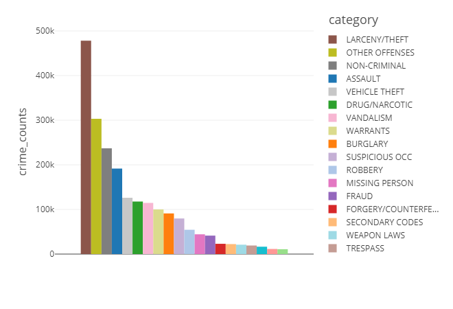
   I want to analyze the count of crime of each category here, so there are two ways to do this.

# Display Count of cime using SQL
crimeCategory = spark.sql("SELECT  category, COUNT(*) AS crime_counts FROM sf_crime GROUP BY category ORDER BY crime_counts DESC")
crimes_pd_df = crimeCategory.toPandas()
display(crimeCategory)

# Display Count of crime of each category Using PySpark
crime_category_df = df_opt1.groupby('category').count().orderBy('count',ascending=False)
crime_category_df = crime_category_df.withColumnRenamed('count', 'crime_counts')
crime_category_df = crime_category_df.toPandas()
display(crime_category_df)

Result

Advance Topic: Machine Learning Model

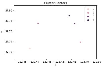
Using KMean Clustering to find the 5 centers in which crimes occur frequently

1. Select Position data X,Y and then Use Interquantile Range method to find outliers of position
   Since KMean Clustering is sensitive to the outlier as it uses mean method to find the center of clusters, we need to remove outliers first.

• Quantile Based method to remove outlier:

The outlier is defined as the data point that drop outside the range [Q1-1.5IQR , Q3+1.5IQR],
where Q1 and Q3 are the first and third quantile of dataset and IQR = Q3-Q1 is the interquantile range.

• API in PySpark to find quantile:

df.approxQuantile(col, probabilities, relativeError):
col: column to find quantile
probabilities: a list of quantile probabilities we want to find. Here I want to find Q1 =0.25 and Q3=0.75
return: the a list values that correspond to the quantile in probabilities list.

# select the positions where crimes occur
crime_cluster_df = df_opt1.where("hasCriminal =true").select(["Hour", "PdDistrict", "X","Y", "DayOfWeek", "category","Resolution","hasCriminal"])
# crime_cluster_df.show()

#Find the Q1, Q 3 Quantile
bounds = {
    c: dict(
        zip(["q1", "q3"], crime_cluster_df.approxQuantile(c, [0.25, 0.75], 0))
    )
    for c in crime_cluster_df.select(["X","Y"]).columns
}

# compute lower bound and upper bound of normal data
for c in bounds:
    iqr = bounds[c]['q3'] - bounds[c]['q1']
    bounds[c]['lower'] = bounds[c]['q1'] - (iqr * 1.5)
    bounds[c]['upper'] = bounds[c]['q3'] + (iqr * 1.5)

2. Remove Outliers based on upper bound and lower bound of quantile

   from pyspark.sql.functions import *
   crime_cluster_df = crime_cluster_df.select(["X","Y"])\
   .where(col("X").between(bounds['X']['lower'], bounds['X']['upper'])) \
   .where(col("Y").between(bounds['Y']['lower'], bounds['Y']['upper']))

   
   

3. Assemble columns into one feature column before training
   In PySpark, we need to put all feature columns into one single feature column before we train the model.

VectorAssembler provides a way to assemble those features into one column.

# ensemble multiple columns into one single feature column for training KMean Clustering
from pyspark.ml.feature import VectorAssembler
vecAssembler = VectorAssembler(inputCols=["X", "Y"], outputCol="features")
crime_cluster_df = vecAssembler.transform(crime_cluster_df.select(["X","Y"]))

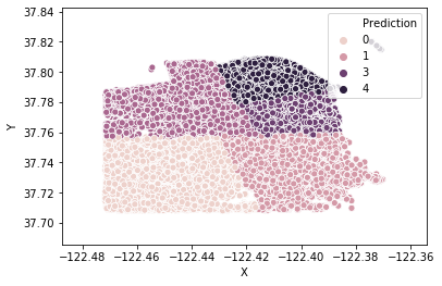
4. KMean Clustering to learn data
   In Machine Learning of PySpark, we need to set the name of feature column to “features”, otherwise, set featuresCol="column-name" to select which feature column to learn in dataframe

# Training KMean clustering
from pyspark.ml.clustering import BisectingKMeans
K=5
bkm = BisectingKMeans(k=K, minDivisibleClusterSize=1.0)
model = bkm.fit(crime_cluster_df)
# predict at one single point
# print(model.predict(crime_cluster_df.head().features))

# predict clusters
# Output the prediction to the column called "Prediction"
model.setPredictionCol("Prediction")
transformed = model.transform(crime_cluster_df).select("X","Y", "Prediction")

Result

Summary

This tutorial introduce:

1. List of useful PySpark functions and their basic usage
2. Use SF Crime dataset as a demo to see how to use PySpark to manipulate data and visualize them
3. How to use machine learning model: KMean Clustering in PySpark to learn data. Note: the APIs of ML in PySpark are different from sklearn. Need to Pay attention to the difference.
   

Reference

[1] SparkReader,Writer
[2] PySpark,SQL_module
[3] PySpark,ML_module
[4] PySpark,outlier_detection
[5] logo